install.packages(c("tidyverse", "tidytext", "wordcloud"))
First let’s get the book “Sense & Sensibility” by Jane Austen
library(tidyverse)
library(tidytext)
library(wordcloud)
book <- janeaustenr::austen_books() |>
  filter(book == "Sense & Sensibility")
slice(book, 50:60)
# A tibble: 11 × 2
text book
<chr> <fct>
1 and daughters than for himself or his son;--but to his son, and his Sens…
2 son's son, a child of four years old, it was secured, in such a way, as Sens…
3 to leave to himself no power of providing for those who were most dear Sens…
4 to him, and who most needed a provision by any charge on the estate, or Sens…
5 by any sale of its valuable woods. The whole was tied up for the Sens…
6 benefit of this child, who, in occasional visits with his father and Sens…
7 mother at Norland, had so far gained on the affections of his uncle, by Sens…
8 such attractions as are by no means unusual in children of two or three Sens…
9 years old; an imperfect articulation, an earnest desire of having his Sens…
10 own way, many cunning tricks, and a great deal of noise, as to outweigh Sens…
11 all the value of all the attention which, for years, he had received Sens…1 Tokenization and Word Frequencies
Let’s split the text by words and count their frequencies.
tokens <- book |>
  unnest_tokens(word, text) |>
  count(word, sort = TRUE)
The result shows that there are a lot of words which are not very informative, such as “the”, “and”, “to”, etc.
tokens # A tibble: 6,419 × 2
word n
<chr> <int>
1 to 4116
2 the 4105
3 of 3571
4 and 3490
5 her 2543
6 a 2092
7 i 1998
8 in 1979
9 was 1861
10 it 1755
# ℹ 6,409 more rowswordcloud(words = tokens$word[1:200],
freq = tokens$n[1:200])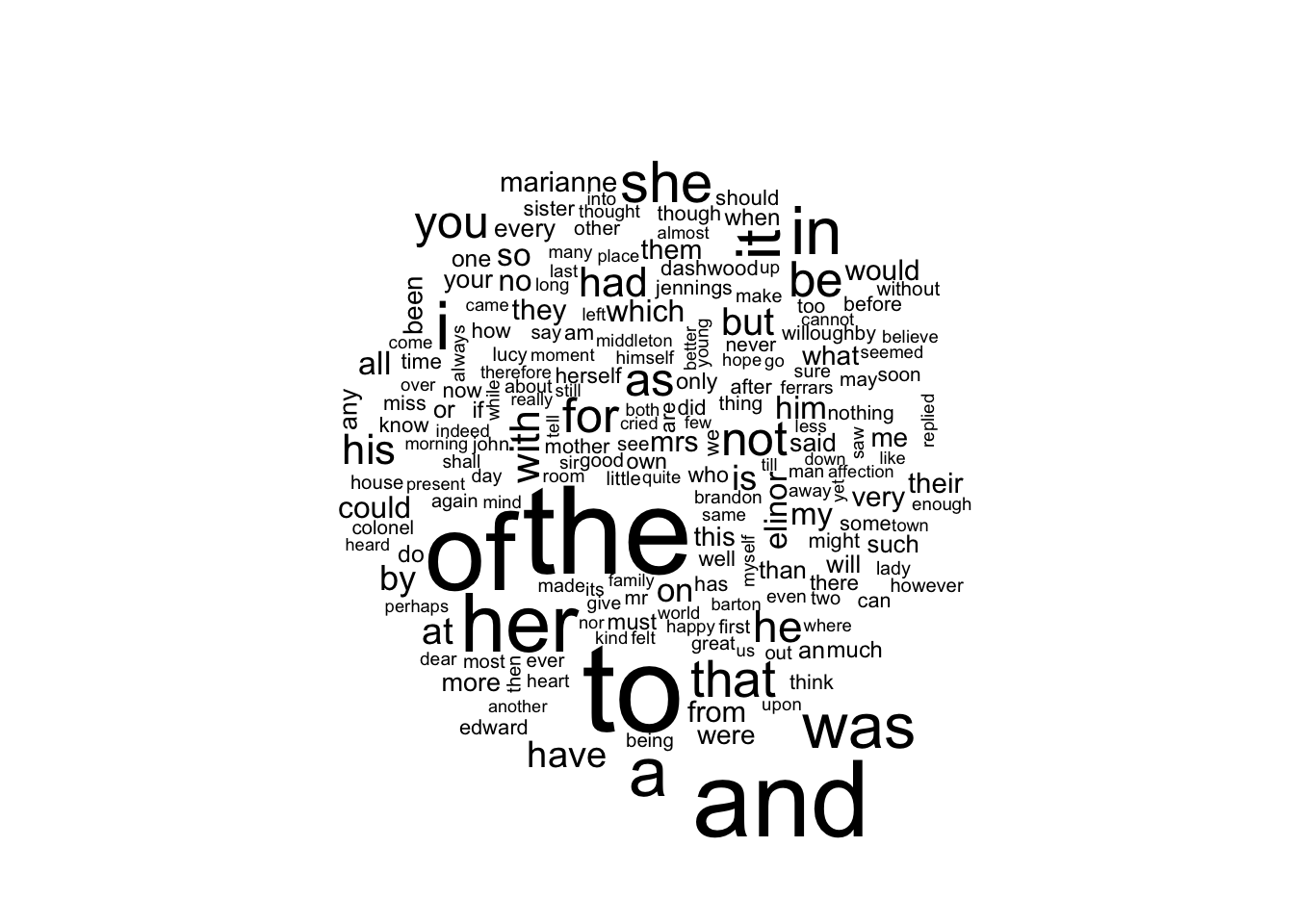
2 Remove stop words
Let’s remove common stop words from the tokens. The tidytext package provides a built-in list of stop words.
clean_tokens <- tokens |>
  anti_join(stop_words, by = "word")
We can see now the informative frequest words in the book:
clean_tokens # A tibble: 5,897 × 2
word n
<chr> <int>
1 elinor 623
2 marianne 492
3 time 239
4 dashwood 231
5 sister 229
6 edward 220
7 mother 213
8 miss 210
9 jennings 199
10 willoughby 181
# ℹ 5,887 more rowswordcloud(words = clean_tokens$word[1:30],
freq = clean_tokens$n[1:30])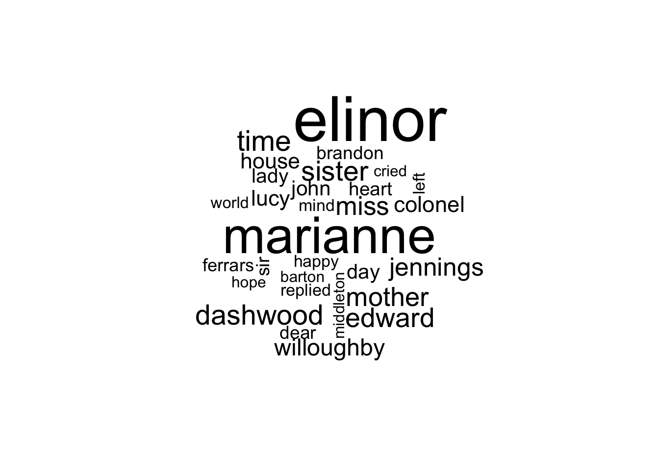
3 Bigram Analysis
Some times, we want to look at pairs of words (bigrams) instead of single words. This can help us understand common phrases or terms used in the text.
bigrams <- book |>
  unnest_tokens(bigram, text, token = "ngrams", n = 2) |>
  count(bigram, sort = TRUE) |>
  separate(bigram, into = c("word1", "word2"), sep = " ", remove = FALSE) |>
  # remove if both word are stop words
  filter(!word1 %in% stop_words$word & !word2 %in% stop_words$word)

bigrams
# A tibble: 4,974 × 4
bigram word1 word2 n
<chr> <chr> <chr> <int>
1 <NA> <NA> <NA> 2199
2 colonel brandon colonel brandon 96
3 sir john sir john 94
4 lady middleton lady middleton 75
5 miss dashwood miss dashwood 55
6 john dashwood john dashwood 34
7 thousand pounds thousand pounds 27
8 replied elinor replied elinor 26
9 cried marianne cried marianne 25
10 miss steeles miss steeles 25
# ℹ 4,964 more rows🎉 Yee-haw! You’ve reached the end of this exercise! You are smashing! Proceed to …