simulate: proof of concept R-package

A proof of concept of parametric simulation framework to generate complex multivariate and multilevel data

This blog post shows a proof of concept for a simulation framework, wrapped into (undocumented) R-package simulate. Let’s take the penguins data from the palmerpenguins package as an example data. You can see the form of the data below if you’re not familiar with it.

library(tidyverse)
library(palmerpenguins)
library(simulate)
theme_set(theme_bw())
set.seed(2022-02-24)
str(penguins)

tibble [344 × 8] (S3: tbl_df/tbl/data.frame)
 $ species          : Factor w/ 3 levels "Adelie","Chinstrap",..: 1 1 1 1 1 1 1 1 1 1 ...
 $ island           : Factor w/ 3 levels "Biscoe","Dream",..: 3 3 3 3 3 3 3 3 3 3 ...
 $ bill_length_mm   : num [1:344] 39.1 39.5 40.3 NA 36.7 39.3 38.9 39.2 34.1 42 ...
 $ bill_depth_mm    : num [1:344] 18.7 17.4 18 NA 19.3 20.6 17.8 19.6 18.1 20.2 ...
 $ flipper_length_mm: int [1:344] 181 186 195 NA 193 190 181 195 193 190 ...
 $ body_mass_g      : int [1:344] 3750 3800 3250 NA 3450 3650 3625 4675 3475 4250 ...
 $ sex              : Factor w/ 2 levels "female","male": 2 1 1 NA 1 2 1 2 NA NA ...
 $ year             : int [1:344] 2007 2007 2007 2007 2007 2007 2007 2007 2007 2007 ...

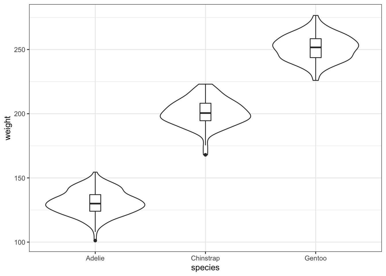
Let’s now say you want to simulate a new response called weight which you assume is normally distributed where the mean is a function of species and variance is 10. We want to specify the mean separately by species such that Adelie, Chinstrap and Gentoo are 130kg, 200kg and 250kg respectively (These numbers are totally made up!!! And probably way heavey for a penguin?).

sim1 <- penguins %>% 
  simulate(weight = sim_normal(~species, 10) %>% 
             params("mean", species = c("Adelie"    = 130,
                                        "Chinstrap" = 200,
                                        "Gentoo"    = 250)))

Let’s visualise to see if the weight was simulated as expected:

ggplot(sim1, aes(species, weight)) +
  geom_violin() +
  geom_boxplot(width = 0.1)

You can make other parameters, like the standard deviation, as a function of species as well.

sim2 <- penguins %>% 
  simulate(weight = sim_normal(~species, ~species) %>% 
             params("mean", species = c("Adelie"    = 130,
                                        "Chinstrap" = 200,
                                        "Gentoo"    = 250)) %>% 
             params("sd", species = c("Adelie"    = 10,
                                      "Chinstrap" = 40,
                                      "Gentoo"    = 100) ))

And here’s the visualisation:

ggplot(sim2, aes(species, weight)) +
  geom_violin() +
  geom_boxplot(width = 0.1)

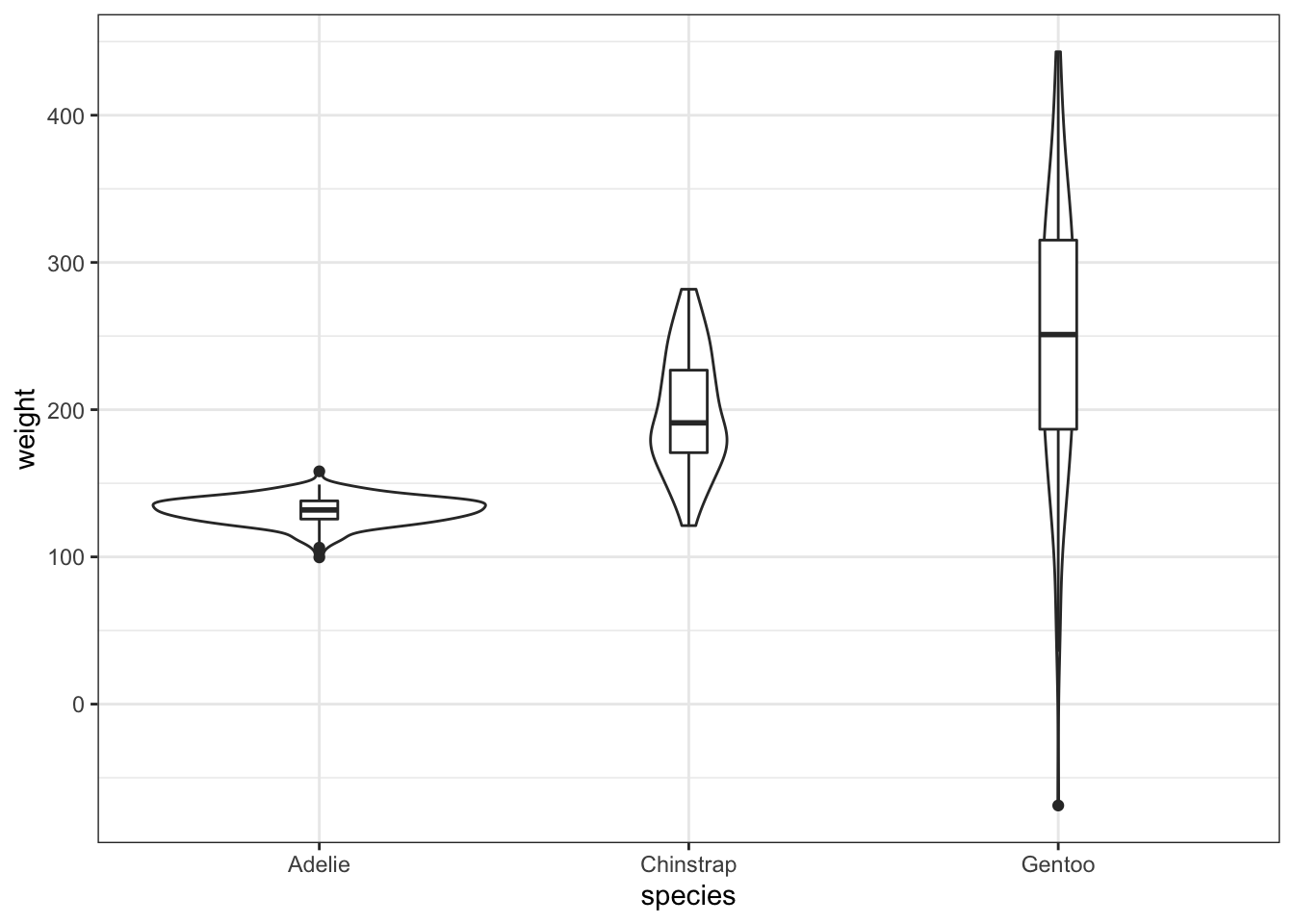
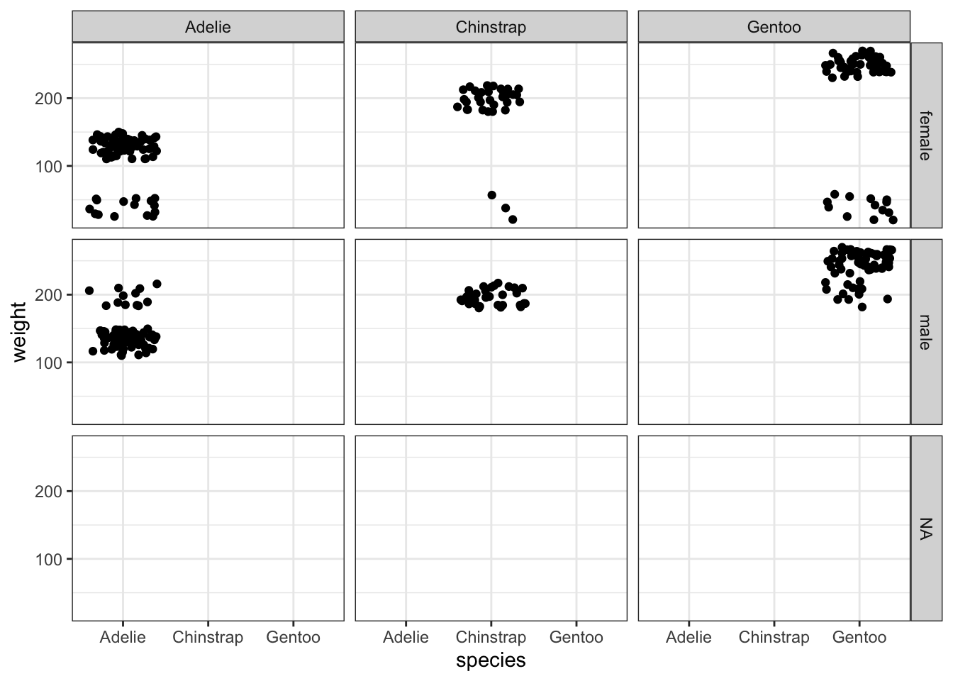
Okay one more before I call it a night. sim_form is a fixed function structure here and I’m simulating weight as a mixture distribution – the weight is either based on the sex or the species (perhaps simulating a situation where some genes aren’t expressed more based on sex sometimes, and sometimes more based on species?? These simulations are just made up.)

sim3 <- penguins %>% 
  simulate(weight = sim_form(~p[1] * sex + p[2] * species) %>% 
             params(species = c("Adelie"    = 130,
                                "Chinstrap" = 200,
                                "Gentoo"    = 250),
                    # it can be unnamed as well
                    sex = c(40, 200),
                    # or specify a distribution
                    p = sim_multinominal(1, c(0.2, 0.8))))

Note: the plot below is jittered so you can see all the points.

ggplot(sim3, aes(species, weight)) +
  geom_jitter() + 
  facet_grid(sex ~ species)

The multivariate part is not shown but a keen user may find how this is envisioned at the moment if you dig deep into the source code… Hint: there is a .cor function to feed in a correlation matrix.