👩🏻‍💻 Emi Tanaka @ Monash University

• emi.tanaka@monash.edu
• @statsgen
• github.com/emitanaka
• emitanaka.org

21st November 2022 ADSN Conference 2022

Experiments are essential

But what does it involve?

The Originator of an Experiment

• What diet lowers insulin?
• Is the lockout laws effective to reduce alcohol-fuelled violence?
• Which brand of washing powder is most effective for cleaning clothes?
• How much fertilizer should you use for optimal crop yield?

The “domain expert” drives the experimental objective and has the intricate knowledge about the subject area

Stick person images by OpenClipart-Vectors from Pixabay

The Designer of the Experiment

Let there be an experimental design!

The “statistican” creates the experimental design layout after taking into account the statistical and practical constraints.

The Executor of the Experiment

The “technician” carries out the experiment and collects the data.

The Digester of the Experiment

The “analyst” analyses the data after the data is collected.

The actors are purely illustrative

Roles may be fuzzy

In practice:

• multiple people can take on each role,
• one person can take on multiple roles, and/or
• a person in the role may not specialise in that role.

Human communication is complex

Source: xkcd “Communication” https://xkcd.com/1028/

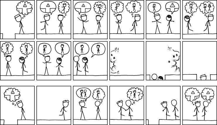
Interdisciplinary communication is challenging

Training in experimental design

• Often about the analysis of experimental data rather than design
• Tendancies to present a menu of named experimental designs (e.g. Randomised Complete Block Design, Split-Plot Design, Balanced Incomplete Block Design, Latin Square Design, etc)
• Communication strategies in formulating alternative views are often not part of the training or teaching

Literature and software in experimental design

• Often product-oriented rather than process-oriented
• Tendencies to focus on algorithmic aspects, e.g. 
  • constrained randomisation and selection of treatments,
  • model- or optimisation-based designs,
  • adaptive designs, and
  • space filling designs.
• Experimental context is stripped away or is an after-thought.

Tanaka & Amaliah (2022) Current state and prospects of R-packages for the design of experiments. arxiv.org/abs/2206.07532

Demonstrations

agricolae package

“Recipe”-based experimental designs

diets <- c("Control", "High-sugar", "High-fat")

# Completely Randomised Design
agricolae::design.crd(trt = diets, r = 10) 
# Randomised Complete Block Design
agricolae::design.rcbd(trt = diets, r = 10) 

exercise <- c("Yes", "No")

# Factorial design
agricolae::design.ab(trt = c(length(diets), length(exercise)), r = 10) 
# Split-plot design
agricolae::design.split(trt1 = diets, trt2 = exercise, r = 10) 

AlgDesign package

“Recipe”-based optimal designs

diets <- c("Control", "High-sugar", "High-fat")
exercise <- c("Yes", "No")
data <- expand.grid(trt1 = diets, trt2 = exercise, rep = 1:10)

# Optimal design with Federov's exchange algorithm
AlgDesign::optFederov(~ trt1 + trt2 + trt1:trt2, 
                      data = data,
                      nTrials = 40,
                      criterion = "D")

# Optimal design via Monte Carlo
AlgDesign::optMonteCarlo(~ trt1 + trt2 + trt1:trt2, 
                         data = data,
                         nTrials = 40,
                         criterion = "D")

But what are the units??

Towards a unified language

Grammarware

• “Grammarware” refers to grammar and grammar-dependent software
• A grammar combines a limited set of words under shared linguistic rules to compose unlimited number of proper sentences.
• Some notable grammarware in statistics include:
  • “The Grammar of Graphics” by Wilkinson interpreted as ggplot2 in R, Gadfly in Julia and plotnine in Python
  • A “Grammar of Data Manipulation” in dplyr, inherited much from the SQL syntax
• The Grammar of Experimental Designs (WIP)
  emitanaka.org/edibble-book

The Grammar of Experimental Designs

(WIP) emitanaka.org/edibble-book

• A computational framework to specify experimental designs based on an objective-oriented programming system that encapsulates the experimental structure and context in a cognitive approach.
• Aims to engage human cognition by building experimental designs with modular functions that modify a targetted, singular element of the experimental design.

Hypothesis:

1.   increasing plant diversity leads to increasing soil microbial biomass and enzyme activity,
2.   higher temperature decreases soil microbial biomassand enzyme activity, and
3.   higher plant diversity buffers effects of elevated temperature on soil microbialbiomass and enzyme activity.

MATERIALS AND METHODS

Experimental design

The present study took place in the BAC experiment site established at the Cedar Creek Ecosystem Science Reserve, Minnesota, USA. The site occurs on a glacial outwash plain with sandy soils. Mean temperature during the growing season (April–September) was 15.98°C in 2011 and 17.18°C in 2012. Precipitation during the growing season was 721 mm in 2011. The growing season in 2012 was considerably drier, with 545 mm rainfall.

Experimental plots (9×9 m) were planted in 1994 and 1995 with different plant communities spanning a plant diversity gradient of one, four, and 16 species, which were randomly chosen from the species listed below (Tilman et al. 2001). The grassland prairie species belonged to one of five plant functional groups: C₃ grasses (Agropyron smithii Tydb., Elymus canadensis L., Koeleria cristata (Ledeb.) Schult., Poa pratensis L.), C₄ grasses (Andropogon gerardii Vitman., Panicum virgatum L., Schizachyrium scoparium (Michx.) Nash, Sorghas-trum nutans (L.) Nash), legumes (Amorpha canescens Pursh., Lespedeza capitata Michx., Lupinus perennis L., Petalostemum purpureum (Vent.) Rydb., Petalostemum villosum Spreng.), nonlegume forbs (Achillea millefolium L., Asclepias tuberosa L., Liatris aspera Michx., Monarda fistulosa L., Soldidago rigida L.), and woody species (Quercus ellipsoidalis E. J. Hill, Quercus macro-carpa Michx.). The individuals of those two woody species (Quercus spp.), which were small in size and rare because of low survival, were removed from all plots in which they occurred in 2010.

In addition to the manipulation of plant diversity,the plots were divided into three subplots (2.5×3.0 m). Heat treatments were applied from March to November each year, beginning in 2009, using infrared lamps 1.8 m above ground emitting 600 W (which caused a 1.5°C increase in soil temperature for vegetation-freesoils) and 1200 W (which caused a 3°C increase; Valpine and Harte 2001, Kimball 2005, Whittingtonet al. 2013) to increase the surface soil temperature of each subplot (see Plate 1). To account for possible shading effects, metal flanges and frames were hungover control subplots. An average across all vegetated plots, temperature manipulations elevated soil temperature at 1 cm depth by 1.18°C in the low warming (+1.5°C) treatment and by 2.69°C in the high warming (+3°C) treatment, and at 10 cm depth temperature by 1.00°C in the low warming (+1.5°C) treatment and by 2.16°C in the high warming (+3°C) treatment.

Soil samples of three subplots in each of 27 experimental plots were taken; due to technical difficulties we could only analyze 66 samples out of 81 existing subplots (monoculture, 10 replicates in ambient +0°C treatment, eight replicates in +1.5°C treatment, nine replicates in +3°C treatment; four species mixture, six replicates in ambient +0°C treatment, six replicates in +1.5°C treatment, seven replicates in +3°C treatment; 16 species mixture, six replicates in ambient +0°C treatment, six replicates in +1.5°C treatment, eight replicates in +3°C treatment). The BAC plots are a representative subset of the plots in the biodiversity experiment E120 at Cedar Creek, which were assembled as random draws of a given number of species from the species pool (Zak et al. 2003). Given low heterogeneity of soil abiotic conditions at the start of the experiment, the experiment was not blocked.

Experimental design with edibble

Experimental design (condensed version)

• Experimental plots were planted with different plant communities spanning a plant diversity gradient of one, four, and 16 species, which were randomly chosen from the species listed (5 plant functional groups – 19 species in total)
• Plots were divided into three subplots
• Heat treatments were applied to subplots emitting 600 W which caused a 1.5°C increase in soil temperature for vegetation-free soils) and 1200 W (which caused a 3°C increase) (control with 0°C included)
• Soil samples of three subplots in each of 27 experimental plots were taken
• Given low heterogeneity of soil abiotic conditions at the start of the experiment, the experiment was not blocked.

library(edibble)
design("Steinauer et al. 2015")

Experimental design with edibble

Experimental design (condensed version)

• Experimental plots were planted with different plant communities spanning a plant diversity gradient of one, four, and 16 species, which were randomly chosen from the species listed (5 plant functional groups – 19 species in total)
• Plots were divided into three subplots
• Heat treatments were applied to subplots emitting 600 W which caused a 1.5°C increase in soil temperature for vegetation-free soils) and 1200 W (which caused a 3°C increase) (control with 0°C included)
• Soil samples of three subplots in each of 27 experimental plots were taken
• Given low heterogeneity of soil abiotic conditions at the start of the experiment, the experiment was not blocked.

library(edibble)
design("Steinauer et al. 2015") %>% 
  set_trts(diversity = c(1, 4, 16))

Experimental design with edibble

Experimental design (condensed version)

• Experimental plots were planted with different plant communities spanning a plant diversity gradient of one, four, and 16 species, which were randomly chosen from the species listed (5 plant functional groups – 19 species in total)
• Plots were divided into three subplots
• Heat treatments were applied to subplots emitting 600 W which caused a 1.5°C increase in soil temperature for vegetation-free soils) and 1200 W (which caused a 3°C increase) (control with 0°C included)
• Soil samples of three subplots in each of 27 experimental plots were taken
• Given low heterogeneity of soil abiotic conditions at the start of the experiment, the experiment was not blocked.

library(edibble)
design("Steinauer et al. 2015") %>% 
  set_trts(diversity = c(1, 4, 16)) %>% 
  set_units(plot = 27,
            subplot = nested_in(plot, 3))

Experimental design with edibble

Experimental design (condensed version)

• Experimental plots were planted with different plant communities spanning a plant diversity gradient of one, four, and 16 species, which were randomly chosen from the species listed (5 plant functional groups – 19 species in total)
• Plots were divided into three subplots
• Heat treatments were applied to subplots emitting 600 W which caused a 1.5°C increase in soil temperature for vegetation-free soils) and 1200 W (which caused a 3°C increase) (control with 0°C included)
• Soil samples of three subplots in each of 27 experimental plots were taken
• Given low heterogeneity of soil abiotic conditions at the start of the experiment, the experiment was not blocked.

library(edibble)
design("Steinauer et al. 2015") %>% 
  set_trts(diversity = c(1, 4, 16)) %>% 
  set_units(plot = 27,
            subplot = nested_in(plot, 3)) %>% 
  set_trts(heat = c("0°C", "1.5°C", "3°C"))

Experimental design with edibble

Experimental design (condensed version)

• Experimental plots were planted with different plant communities spanning a plant diversity gradient of one, four, and 16 species, which were randomly chosen from the species listed (5 plant functional groups – 19 species in total)
• Plots were divided into three subplots
• Heat treatments were applied to subplots emitting 600 W which caused a 1.5°C increase in soil temperature for vegetation-free soils) and 1200 W (which caused a 3°C increase) (control with 0°C included)
• Soil samples of three subplots in each of 27 experimental plots were taken
• Given low heterogeneity of soil abiotic conditions at the start of the experiment, the experiment was not blocked.

library(edibble)
design("Steinauer et al. 2015") %>% 
  set_trts(diversity = c(1, 4, 16)) %>% 
  set_units(plot = 27,
            subplot = nested_in(plot, 3)) %>% 
  set_trts(heat = c("0°C", "1.5°C", "3°C")) %>% 
  allot_trts(diversity ~ plot,
                  heat ~ subplot)

Experimental design with edibble

Experimental design (condensed version)

• Experimental plots were planted with different plant communities spanning a plant diversity gradient of one, four, and 16 species, which were randomly chosen from the species listed (5 plant functional groups – 19 species in total)
• Plots were divided into three subplots
• Heat treatments were applied to subplots emitting 600 W which caused a 1.5°C increase in soil temperature for vegetation-free soils) and 1200 W (which caused a 3°C increase) (control with 0°C included)
• Soil samples of three subplots in each of 27 experimental plots were taken
• Given low heterogeneity of soil abiotic conditions at the start of the experiment, the experiment was not blocked.

library(edibble)
design("Steinauer et al. 2015") %>% 
  set_trts(diversity = c(1, 4, 16)) %>% 
  set_units(plot = 27,
            subplot = nested_in(plot, 3)) %>% 
  set_trts(heat = c("0°C", "1.5°C", "3°C")) %>% 
  allot_trts(diversity ~ plot,
                  heat ~ subplot) %>% 
  # guessing treatment were randomly allocated
  assign_trts(order = "random", seed = 2022)

Experimental design with edibble

Experimental design (condensed version)

• Experimental plots were planted with different plant communities spanning a plant diversity gradient of one, four, and 16 species, which were randomly chosen from the species listed (5 plant functional groups – 19 species in total)
• Plots were divided into three subplots
• Heat treatments were applied to subplots emitting 600 W which caused a 1.5°C increase in soil temperature for vegetation-free soils) and 1200 W (which caused a 3°C increase) (control with 0°C included)
• Soil samples of three subplots in each of 27 experimental plots were taken
• Given low heterogeneity of soil abiotic conditions at the start of the experiment, the experiment was not blocked.

library(edibble)
design("Steinauer et al. 2015") %>% 
  set_trts(diversity = c(1, 4, 16)) %>% 
  set_units(plot = 27,
            subplot = nested_in(plot, 3)) %>% 
  set_trts(heat = c("0°C", "1.5°C", "3°C")) %>% 
  allot_trts(diversity ~ plot,
                  heat ~ subplot) %>% 
  # guessing treatment were randomly allocated
  assign_trts(order = "random", seed = 2022) %>% 
  serve_table()

This is in fact a split-plot design!

Why edibble?

• Semantics of the syntactic sugar are aligned with basic terms in experimental design (i.e. code can be used for communication that captures user intention).
• Experimental structure are built up step-by-step:
  • internal syntax allows for an incomplete experimental structure, and
  • external syntax makes it easy to modify or replace a single step instead of redoing whole structure.
• A number of downstream benefits, e.g. automated visualisations, setting records/responses, setting expectations of records, simulating records, exporting data with data validation.

Automated visualisation of edibble designs

• deggust R package automatically translates edibble designs as a ggplot object.

library(edibble)
des <- design("Steinauer et al. 2015") %>% 
  set_trts(diversity = c(1, 4, 16)) %>% 
  set_units(plot = 27,
            subplot = nested_in(plot, 3)) %>% 
  set_trts(heat = c("0°C", "1.5°C", "3°C")) %>% 
  allot_trts(diversity ~ plot,
                  heat ~ subplot) %>% 
  assign_trts(order = "random", seed = 2022) %>% 
  serve_table()

deggust::autoplot(des, aspect_ratio = 1.5)

An authentic example

A conversation on Mastodon (similar to Twitter)

@emitanaka Hi, I looked at your edibble package. Is it possible to create designs with repeated measurements? I didn’t see them in your vignette or book draft. thx!

Hi! In terms of repeated measurements, I assume there is no cross-over treatment allocation? If the treatment remains the same for each subject, then repeated measures (to me) is just a special case of multivariate experimental data (so design is not affected, but you have more than one response per subject). So in edibble, the code may be something like attached. Does that help?

library(edibble)
design("Repeated measures experiment") %>% 
  set_units(sex = c("F", "M"), 
            # 10 subject per sex
            subject = nested_in(sex, 10)) %>% 
  set_trts(treatment = c("A", "B")) %>% 
  allot_trts(treatment ~ subject) %>%
  # this is essentially like a randomised complete block design 
  assign_trts("random") %>% 
  # 10 repeated measurements let's say per subject
  set_rcrds_of(subject = paste0("response", 1:10)) %>% 
  serve_table()

Hi, thanks for your reply. I am thinking of designs in cognitive neuroscience, in which we often test only 1 group of participants with multiple within-subject factors. In that case, simply repeating treatments is not correct (though one can construct something like your last line for multiple factors). But I was more thinking of an explicit definition of factors as repeat or non-repeat.

Would you have a good reference of the design that you can point me to? It sounds like you are allocating different treatments at different times/sessions, in this case you need to think of time/session as a unit. I attach the edibble code for the design in your paper here from the way I interpreted it. Does that look right to you?

library(edibble)
design("Fuchs & Heed (2022)") %>% 
  set_units(participant = 22, # originally planned for 25 
            # 2 sessions per participant
            session = nested_in(participant, 2)) %>% 
  set_trts(training = c("congruent", "incongruent")) %>% 
  allot_table(training ~ session)

@emitanaka thank you for your effort of looking through a paper of mine! This does look right, but there would be additional factors that nest within each congruent/incongruent block. For instance, in the paper you looked at, 8 tactile locations, 10 rounds of training (= experimental factor because stimuli change in each round). These things occur both within congruent and incongruent.

library(edibble)
design("Fuchs & Heed (2022)") %>% 
  set_units(participant = 22, # originallly planned for 25
            # 2 sessions per partcipant
            session = nested_in(participant, 2),
            # every session had 10 training session
            round = nested_in(session, 10)) %>% 
  set_trts(training = c("congruent", "incongruent"),
           tactile_location = 1:8) %>% 
  allot_table(training ~ session,
              tactile_location ~ round)

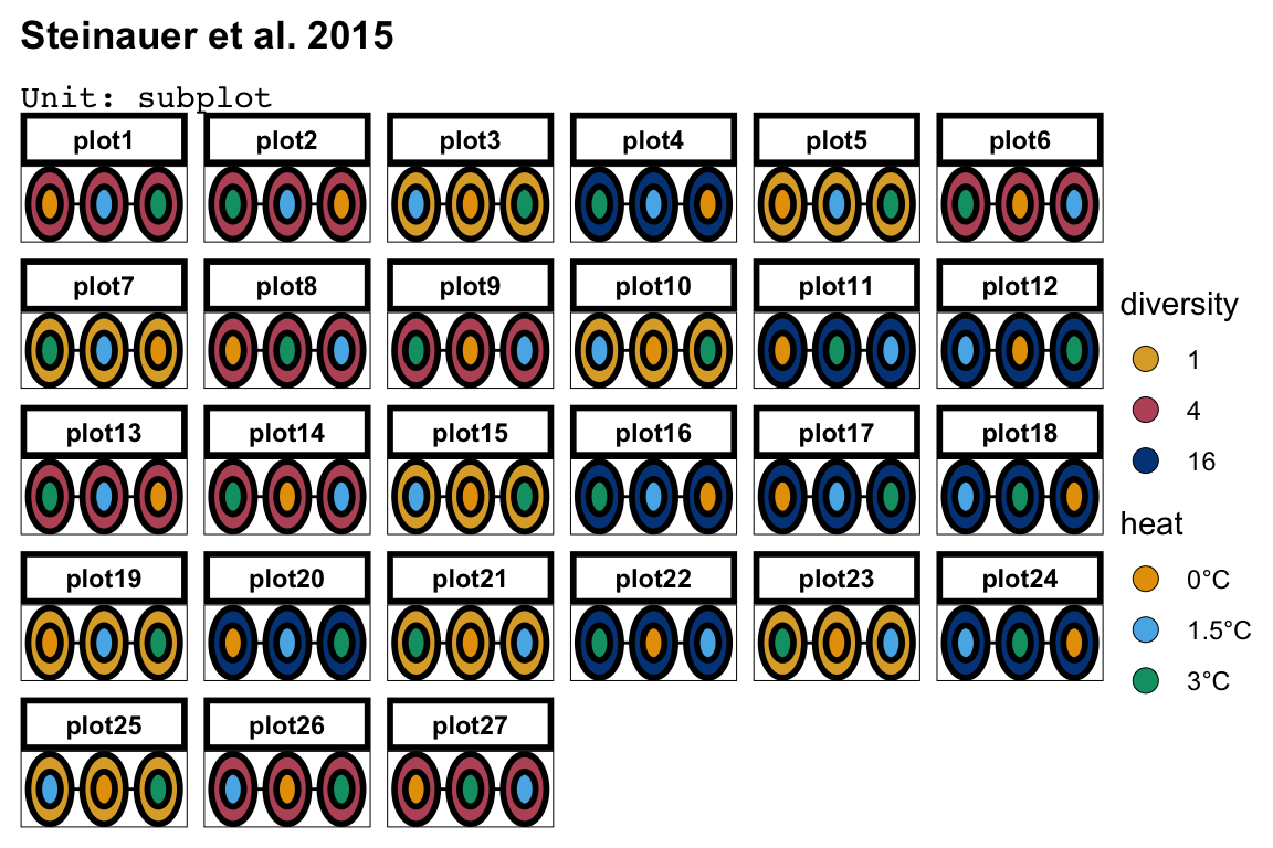
• Experiments are human endeavours often involving complex interdisciplinary communications.
• We can perhaps use an interface design as an unified language to promote a shared understanding.
• edibble is not a silver bullet, but hopefully sheds more clarity.

Slides at emitanaka.org/slides/ADSN2022/

Feedback/comments/questions/requests/collaborations welcome!

github.com/emitanaka/edibble/issues edibble on CRAN, deggust on GitHub

emi.tanaka@monash.edu @statsgen @emitanaka@fosstodon.org github.com/emitanaka