Statistical Communication and Workflow

STAT1003 – Statistical Techniques

Dr. Emi Tanaka

Australian National University

These slides are best viewed on a modern browser like Google Chrome on a desktop or laptop. Some interactive components may require some time to fully load.

Table of contents

• Importing and Exporting Data
  • Data file formats
  • Reading and writing CSV files
  • File paths
  • Folder structure
  • Binary formats
  • Reading Excel sheets
  • Importing through the GUI
  • Formatting or editing data
  • Summary
  • Data import cheatsheet
• What is Quarto?
  • Quarto in a nutshell
  • R Markdown
  • What can you do with Quarto?
  • HTML slides
  • Report
  • Thesis
  • Quarto basics
  • Render to a HTML document
  • Render to a PDF document
  • RStudio Desktop
  • How does it all work?
• Meta Data with YAML
  • YAML - YAML Ain’t Markup Language
  • YAML in Quarto documents
  • YAML with multiple key values and nested keys
  • Values spanning multiple lines
• Text with Markdown
  • Headers
  • Lists
  • Formatting text
  • Inserting images and links
• Dynamic Documents with Data Analysis Code
  • Code chunks
  • Chunk options
  • Quarto (and R Markdown) is not just for R
  • Inline R code
• Cross Reference
  • Bibliography
  • Citing literature
  • Figure references
  • Table references
  • Section references
  • Summary
  • Quarto cheatsheet
• Literate Programming
  • Non-robust workflow
  • A robust, reproducible workflow
  • Analysis framework
  • Statistical value chain
  • Folder structure
  • Sharing your documents

Importing and Exporting Data

Data file formats

• Data are stored as a file, which points to a block of computer memory.
• A file format signals a way to interpret the information stored in the computer memory.
• A file with the extension “csv” (comma-separated values) uses a comma as a delimiter while “tsv” uses tabs as a delimiter.

data.csv

len, supp, dose
4.2, VC, 0.5
11.5, VC, 0.5
...

• A common approach is to have as a text file format where
  • a delimiter (e.g. “,” and tabs) separate columns,
  • the first row (header) corresponds to the names of the variables, and
  • subsequent rows correspond to the values.

Reading and writing CSV files

File paths

• Your file has to be in the right location to be read!
• To point to the right location of the data , you may use
  • a relative path (e.g. data/data.csv) or
  • an absolute path (e.g. C:\\user/myproject/data.csv)

You should avoid using absolute path! Why?

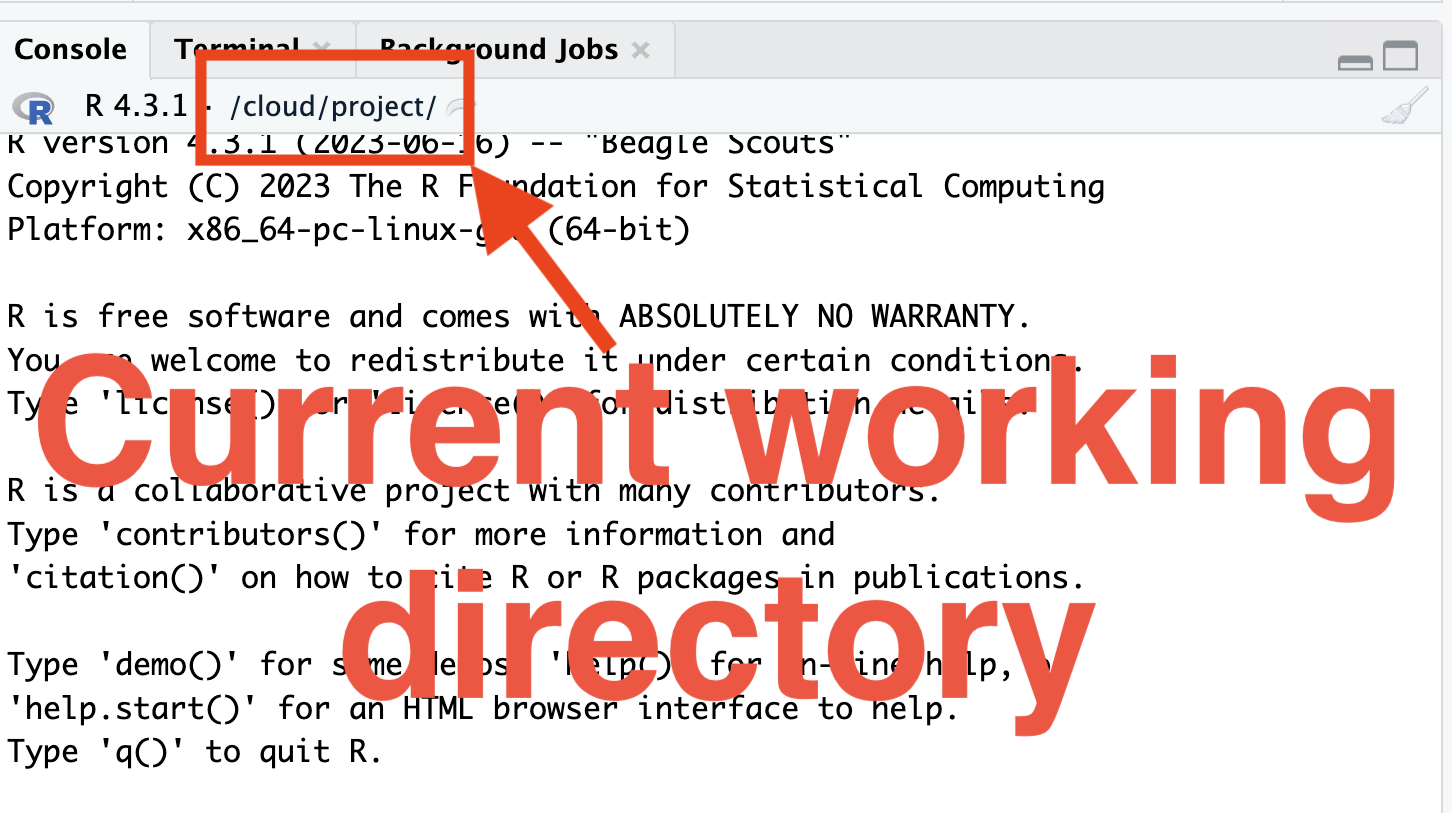
• You can get and set the current path using getwd() and setwd(), respectively.

Folder structure

• Your folder structure depends on the project, but it is generally a good idea to have:
  • a main project folder
  • Within the main project folder, a separate folder for:
    • data
    • code/script/analysis
    • report/paper/outputs.

• Within RStudio, you can create a project file (with an .Rproj extension).
• Double clicking on this .Rproj file launches RStudio Desktop with the current working directory set to the location of the project file.
• You can create this project file by going to RStudio > File > New Project …

Binary formats

• Data can also be stored as a binary format (e.g. .RData, .rda or rds).
• .RData, .rda or rds saves R objects so you don’t need the data to be in a data.frame.
• However, these formats are specific to R and thus not easily portable to other software.

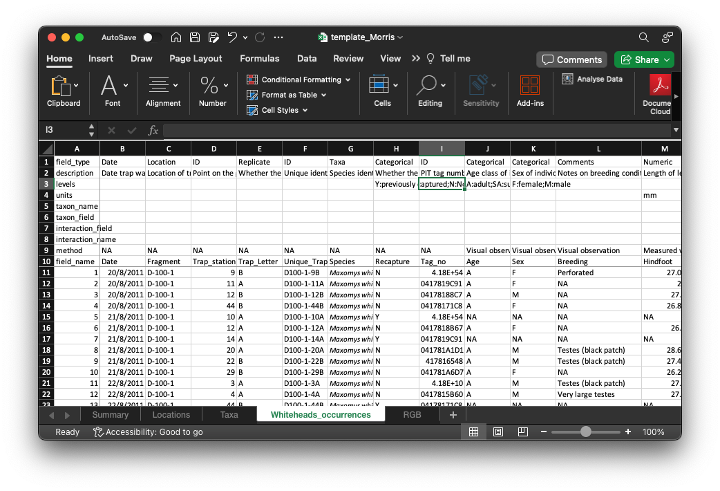
Reading Excel sheets

• Data can also come in a propriety format (e.g. xls and xlsx) – these require special ways to open/view/read it.

data/template_Morris.xlsx

template_Morris.xlsx from Morris & Ewers (2018). Whitehead’s rat morphometrics [Data set]. Zenodo. https://doi.org/10.5281/zenodo.1237733

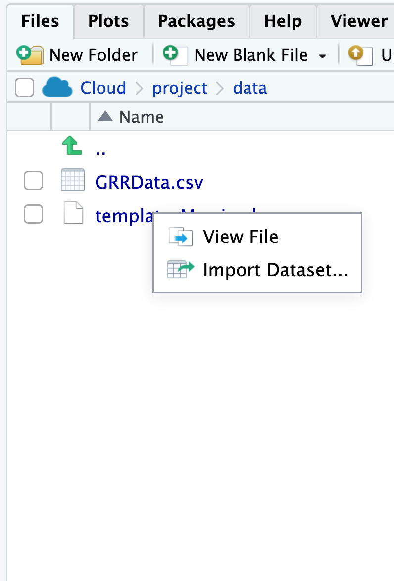
Importing through the GUI

In RStudio Desktop, you can click on the file for importing via GUI.

Formatting or editing data

Unless you are responsible for entering the data, you should never modify the original, stored data (note: exceptions do apply).

• For scientific integrity, any modification to the original data should be recorded in a reproducible manner (e.g. by programming in R!) so that you can trace the exact modifications.

Summary

• You can use readr::read_csv() and readr::write_csv() to read and write CSV files.
• You can use readxl::read_xlsx() to read Excel files.
• Save a single R object using saveRDS() (recommended) and multiple objects using save().
• Load R objects using readRDS() or load().
• In RStudio Desktop, you can click on the file for importing via GUI.
• Set up R Projects and use relative path to data files.
• Don’t ever modify the raw data!

Data import cheatsheet

Data Import Cheatsheet

What is Quarto?

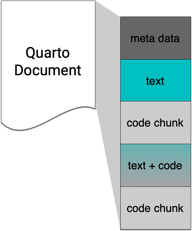
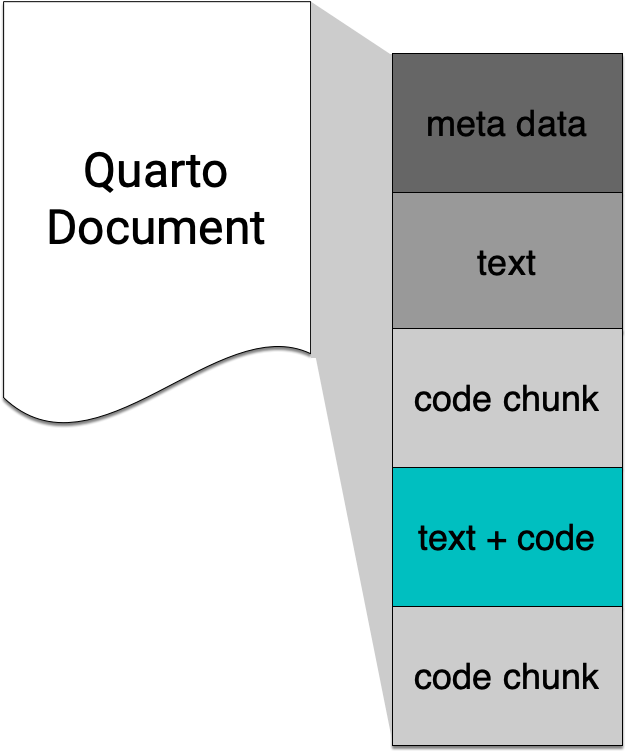
Quarto in a nutshell

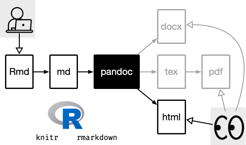
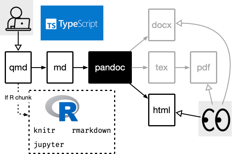
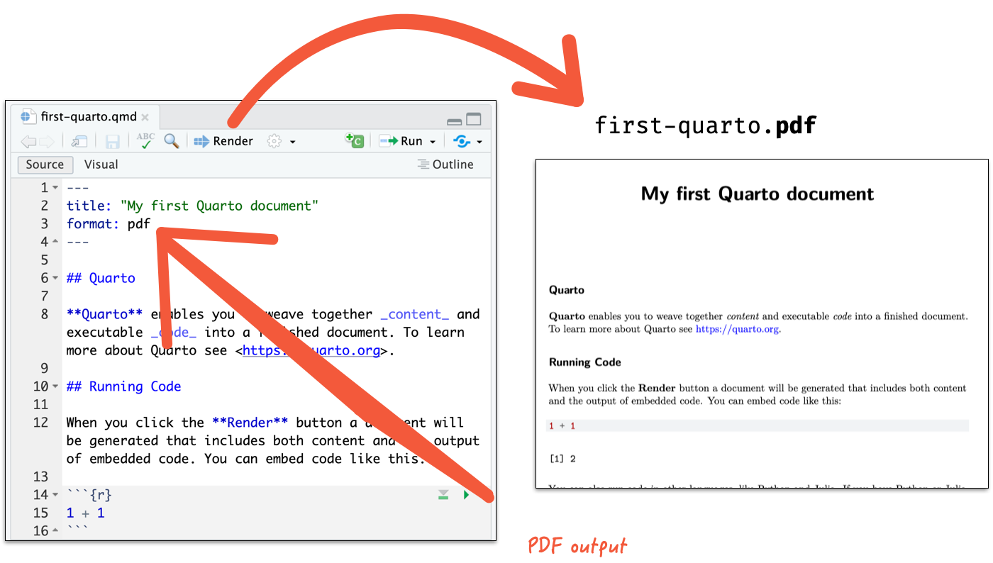
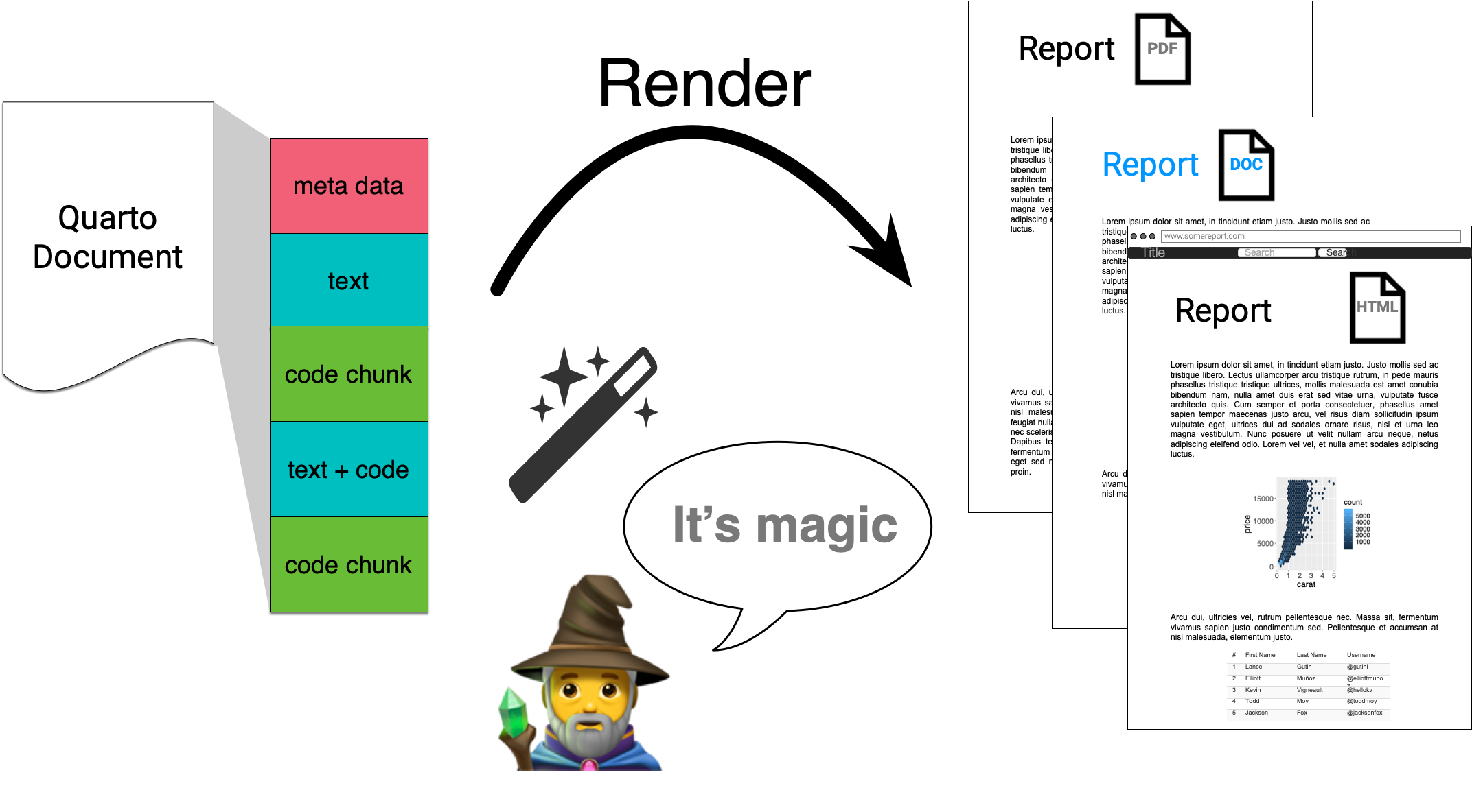
Quarto integrates text + code in one source document with ability to render to many output formats (via Pandoc), e.g. docx, pdf or html.

• Note: Quarto is the next generation of R Markdown.

R Markdown

• Quarto and R Markdown are very similar.
• The same team that created R Markdown created Quarto.
• Quarto supersedes R Markdown so we focus on Quarto.

R Markdown

Quarto

What can you do with Quarto?

There are so many possible output formats you can create with Quarto, including but not limited to:

• Microsoft Word document (.doc, .docx)
• PowerPoint presentation (.pptx)
• Open Document Text (.odt)
• Rich text format (.rtf)
• e-book format (.epub)
• Markdown documents (.md)
• Dashboard (.html)
• Books (.pdf or .html)
• Webpage (.html)
• Websites (collection of web pages)

Primary languages supported:

• R
• Python
• Julia
• Observable

But include engines for many more languages!

HTML slides

These HTML slides are made using Quarto.

Report

These dynamic reports are made using Quarto.

Thesis

This PhD thesis (online and pdf) is made using Quarto.
Available at https://thesis.patrickli.org/

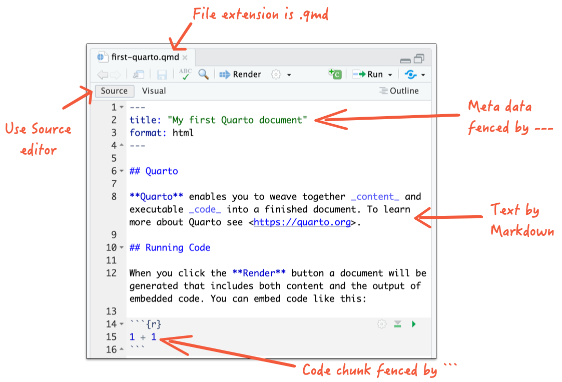
Quarto basics

• If you are not using RStudio Desktop, open with your own editor.

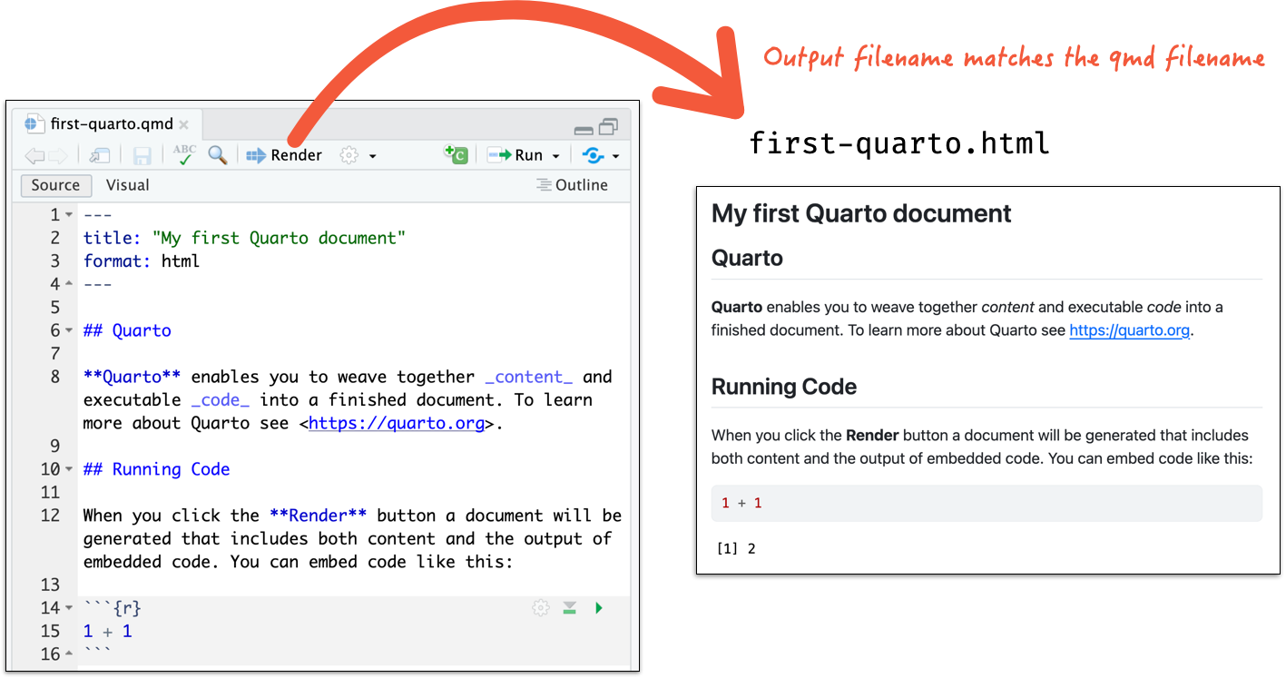
Render to a HTML document

• If you are not using RStudio Desktop, open the terminal and run

quarto render /your/file/location/filename.qmd

Render to a PDF document

• If you are not using RStudio Desktop, open the terminal and run

quarto render /your/file/location/filename.qmd

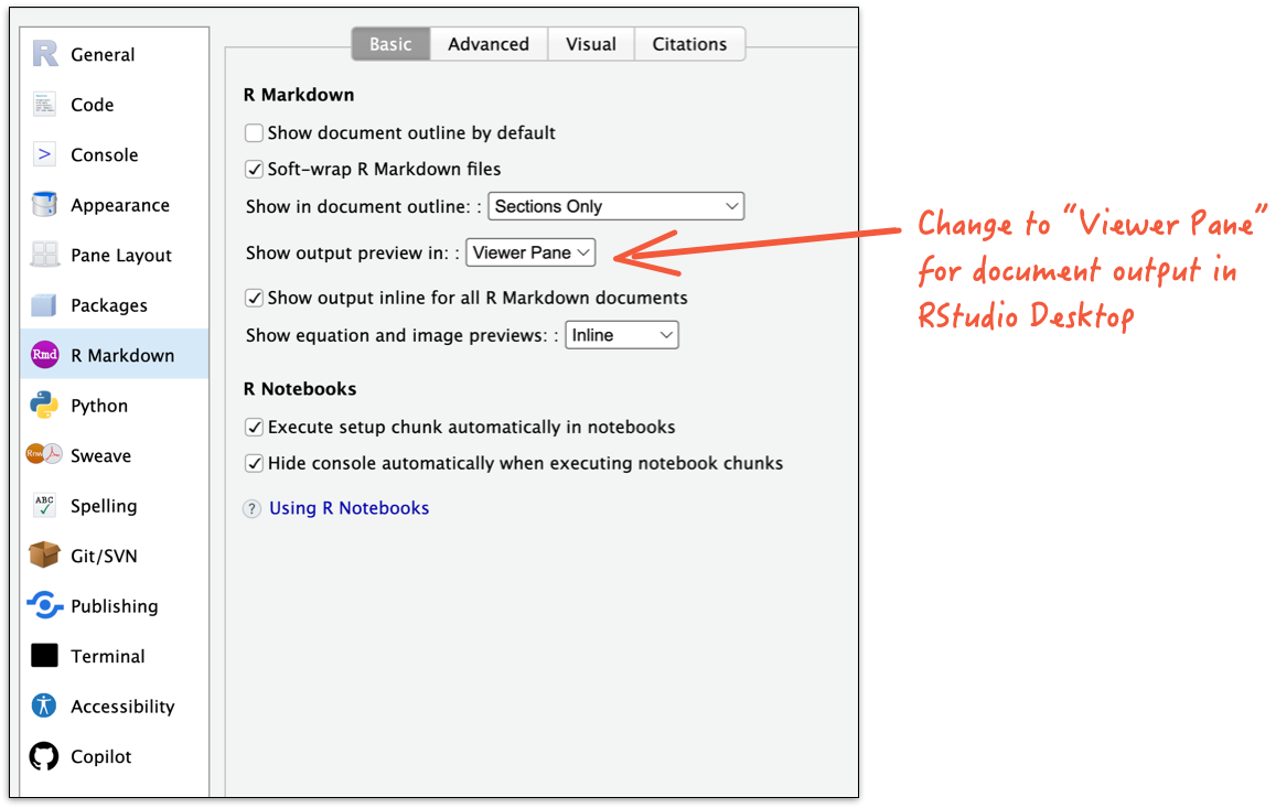
RStudio Desktop

How does it all work?

Quarto via knitr/jupyter: qmd md

Pandoc: md html, pdf, docx

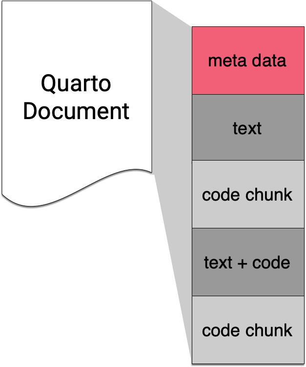
Meta Data with YAML

YAML - YAML Ain’t Markup Language

Basic YAML format to specify document metadata use key-value pairs.

key: value

title: "Meta data with YAML"
subtitle: "The Basics"
author: "Emi Tanaka"
date: "`r Sys.Date()`"
engine: knitr
format: html

• There must be a space after “:”!
• White spaces indicate structure in YAML - don’t use tabs though!
• Same as R, you can comment lines by starting with #.
• YAML is case sensitive.
• Logical values are specified as true or false (all lowercase) in YAML (not TRUE or FALSE like in R).
• If the value is a string and contains special characters (e.g., :, #, -), it should be enclosed in quotes.

YAML in Quarto documents

In Quarto documents, YAML metadata is usually placed at the very top of the document, enclosed by triple dashes ---.

• Some common keys used in Quarto documents:
  • title - the title of the document
  • subtitle - the subtitle of the document
  • author - the author of the document
  • date - the date of the document
  • abstract - a brief summary of the document
  • format - the output format of the document (e.g., html, pdf, docx)

You can find available keys by format at https://quarto.org/docs/reference/

YAML with multiple key values and nested keys

• A key can hold multiple values.

• Multiple values can be listed as a list:

key: 
  - value1
  - value2
  - value3

• Or it can be separated by a comma within a square bracket:

key: [value1, value2, value3]

A key can contain other keys by indenting them below the parent key.

---
format: 
  html:
    toc: true
    theme: sketchy
  pdf: default
---

• What does each of the above keys do?
• The best way to find out is to try them out!

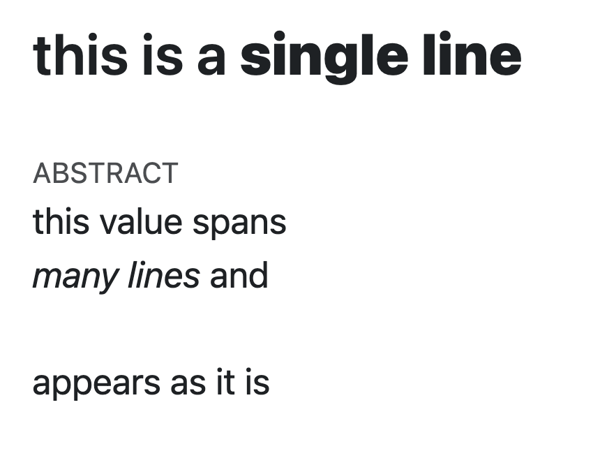
Values spanning multiple lines

A value can span multiple lines in two ways:

• Using the pipe symbol | to preserve line breaks.
• Using the greater-than symbol > to fold lines (line breaks become spaces).

---
title: >
  this is a  
  
  **single line**
  
abstract: |
  | this value spans   
  | *many lines* and      
  | 
  | appears as it is     
  
format: html
---

Text with Markdown

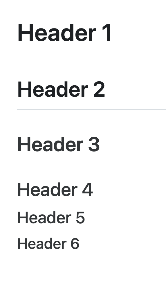
Headers

# Header 1
## Header 2
### Header 3
#### Header 4
##### Header 5
###### Header 6

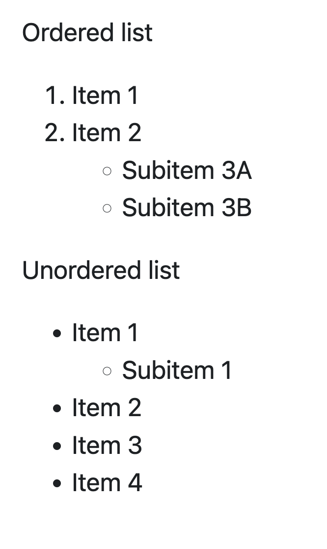
Lists

Ordered list

1. Item 1
2. Item 2
   - Subitem 3A
   - Subitem 3B
  
Unordered list

* Item 1 
  * Subitem 1
* Item 2
- Item 3
- Item 4

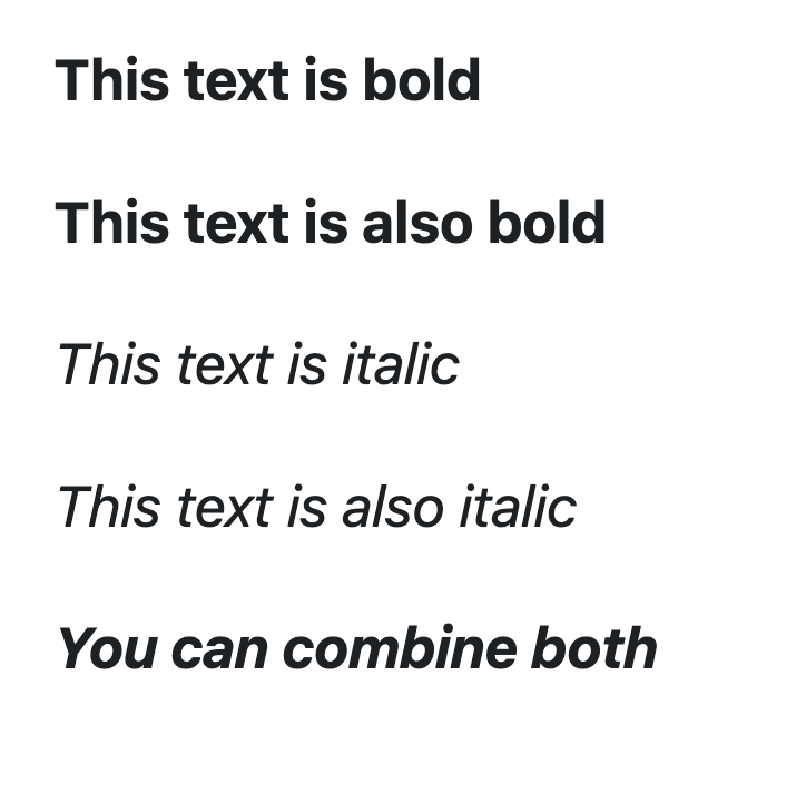
Formatting text

 **This text is bold** 
 
 __This text is also bold__  
 
 *This text is italic* 
 
 _This text is also italic_  
 
 **_You can combine both_** 

Inserting images and links

![Avatar](images/avatar1.jpg){width="50%"}

Check out the
[RSFAS website](https://rsfas.anu.edu.au/)!

<https://rsfas.anu.edu.au/>

Avatar

Check out the RSFAS website!

https://rsfas.anu.edu.au/

RStudio > Help > Markdown Quick Reference

Dynamic Documents with Data Analysis Code

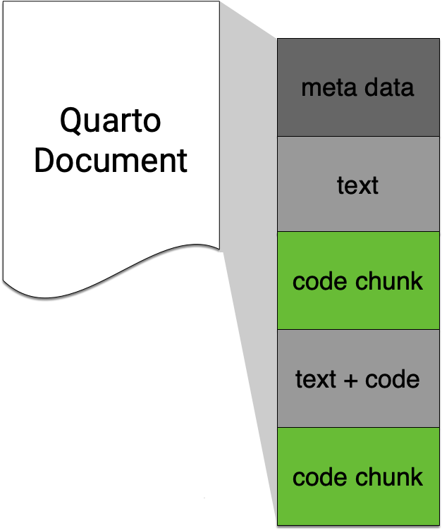
Code chunks

• In Quarto (and R Markdown), code is included in code chunks.
• Code chunks are delimited by triple backticks ``` with the language specified after the opening backticks.

Computation:

```{r}
table(penguins$species)
```

   Adelie Chinstrap    Gentoo 
      152        68       124 

Plotting:

```{r}
library(tidyverse)
ggplot(penguins, aes(body_mass)) + 
      geom_histogram(bins = 30)
```

Chunk options

```{r}
#| label: fig-plot
#| eval: true
#| echo: false
#| fig-width: 5
#| fig-height: 3.5
#| fig-cap: "A scatter plot of bill length and body mass."
library(ggplot2)
ggplot(penguins, aes(bill_len, body_mass)) +
  geom_point()
```

Figure 1: A scatter plot of bill length and body mass.

• label: label for the chunk (for cross-referencing)
• eval: whether to evaluate the code (true or false)
• echo: whether to show the code in the output (true or false)
• fig-width: width of the figure (in inches)
• fig-height: height of the figure (in inches)
• fig-cap: caption for the figure

See more options for the knitr engine at here.

Quarto (and R Markdown) is not just for R

• To use Python, change the language to python:

```{python}
2 * 2 + 3
```

7

• To use Julia, change the language to julia:

```{julia}
3 + 3
```

6

Note: doesn’t work as well with Julia.

The following languages are supported by knitr:

asis, asy, awk, bash, block, block2, bslib, c, cat, cc, coffee, comment, css, ditaa, dot, embed, eviews, exec, fortran, fortran95, gawk, glue, glue_sql, gluesql, go, groovy, haskell, highlight, js, julia, lein, mermaid, mysql, node, octave, ojs, perl, php, psql, python, r, rcpp, rscript, ruby, sas, sass, scala, scss, sed, sh, sql, stan, stata, targets, tikz, verbatim, webr, zsh

Inline R code

`r some_r_code()`

The number of observations in the `ChickWeight` dataset 
is **`r nrow(ChickWeight)`**.

The value of $\pi$ is `r pi`.

The number of observations in the ChickWeight dataset is 578.

The value of \(\pi\) is 3.1415927.

• Note that these inline R command only work if engine: knitr.
• This doesn’t work for other languages.

Cross Reference

Bibliography

• BibTeX citation style format is used to store references in .bib files.
• You can get most BibTeX citation for R packages citation function.

citation("ggplot2")

To cite ggplot2 in publications, please use

  H. Wickham. ggplot2: Elegant Graphics for Data
  Analysis. Springer-Verlag New York, 2016.

A BibTeX entry for LaTeX users is

  @Book{,
    author = {Hadley Wickham},
    title = {ggplot2: Elegant Graphics for Data Analysis},
    publisher = {Springer-Verlag New York},
    year = {2016},
    isbn = {978-3-319-24277-4},
    url = {https://ggplot2.tidyverse.org},
  }

Citing literature

---
bibliography: ref.bib
---

You can cite references like:

- Data analysis was conducted using R [@rstats]
- @ggplot2 was used for plotting.

You can cite references like:

• Data analysis was conducted using R (R Core Team 2025)
• Wickham (2016) was used for plotting.

References

R Core Team. 2025. R: A Language and Environment for Statistical Computing. Vienna, Austria: R Foundation for Statistical Computing. https://www.R-project.org/.

Wickham, Hadley. 2016. Ggplot2: Elegant Graphics for Data Analysis. Springer-Verlag New York. https://ggplot2.tidyverse.org.

• You can cite references in the text using [@key] or @key, where key is the citation key defined in the .bib file.
• References are automatically appended at the end of the document.

ref.bib

@Book{ggplot2,
    author = {Hadley Wickham},
    title = {ggplot2: Elegant Graphics for Data Analysis},
    publisher = {Springer-Verlag New York},
    year = {2016},
    isbn = {978-3-319-24277-4},
    url = {https://ggplot2.tidyverse.org},
  }

@Manual{rstats,
    title = {R: A Language and Environment for Statistical Computing},
    author = {{R Core Team}},
    organization = {R Foundation for Statistical Computing},
    address = {Vienna, Austria},
    year = {2025},
    url = {https://www.R-project.org/},
  }

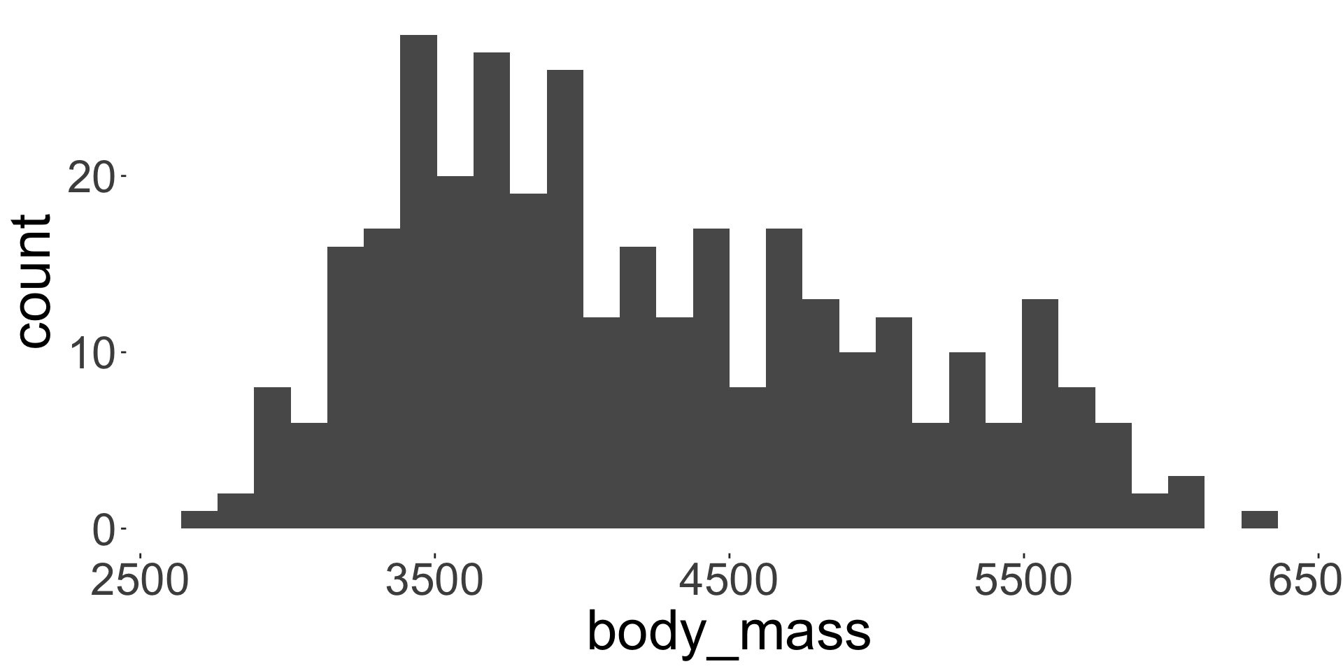
Figure references

The chunk label with prefix fig- can be referenced in text as a figure.

The body mass distribution of penguins is shown in @fig-hist.

```{r}
#| label: fig-hist
#| fig-cap: "Distribution of penguin body mass."
library(ggplot2)
ggplot(penguins, aes(body_mass)) + 
    geom_histogram(bins = 30)
```

The body mass distribution of penguins is shown in Figure 2.

Figure 2: Distribution of penguin body mass.

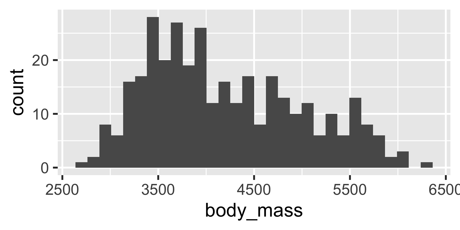
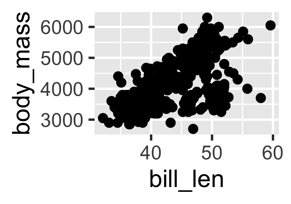
• Above we use the ggplot2 package to create a figure, but you can use base R plotting functions or other packages.

Table references

The chunk label with prefix tbl- can be referenced in text as a table.

```{r}
#| label: tbl-cars
#| tbl-cap: "Summary statistics of penguin body mass by species."
library(dplyr)
penguins |> 
 summarise(Mean = mean(body_mass, na.rm = TRUE),
           SD = sd(body_mass, na.rm = TRUE),
           N = n(),
           .by = species) |> 
 knitr::kable(digits = 1)
```

Table 1: Summary statistics of penguin body mass by species.

species	Mean	SD	N
Adelie	3700.7	458.6	152
Gentoo	5076.0	504.1	124
Chinstrap	3733.1	384.3	68

• Above we use the knitr::kable() function to create a table.
• There are many other packages to create tables, e.g., gt, flextable, kableExtra, etc.

Section references

If you have enabled numbering of sections:

---
number-sections: true
---

then you can refer to them by their label prefixed by sec-.

## Introduction

To see the main results, go to 
@sec-results.

## Results {#sec-results}

The method works!

1 Introduction

To see the main results, go to Section 2.

2 Results

The method works!

Summary

Weave together text, code, and output (figures, tables, etc.) in a single document using Quarto into various output formats (HTML, PDF, Word, etc.).

• Use YAML to control document’s meta data.
• Use Markdown syntax in the body of the document to write content.
• Use R (or Python, Julia, etc.) for data analysis and visualization.
• Focus on writing the content instead of formatting!
• The best guide for Quarto is at https://quarto.org/docs/guide/.

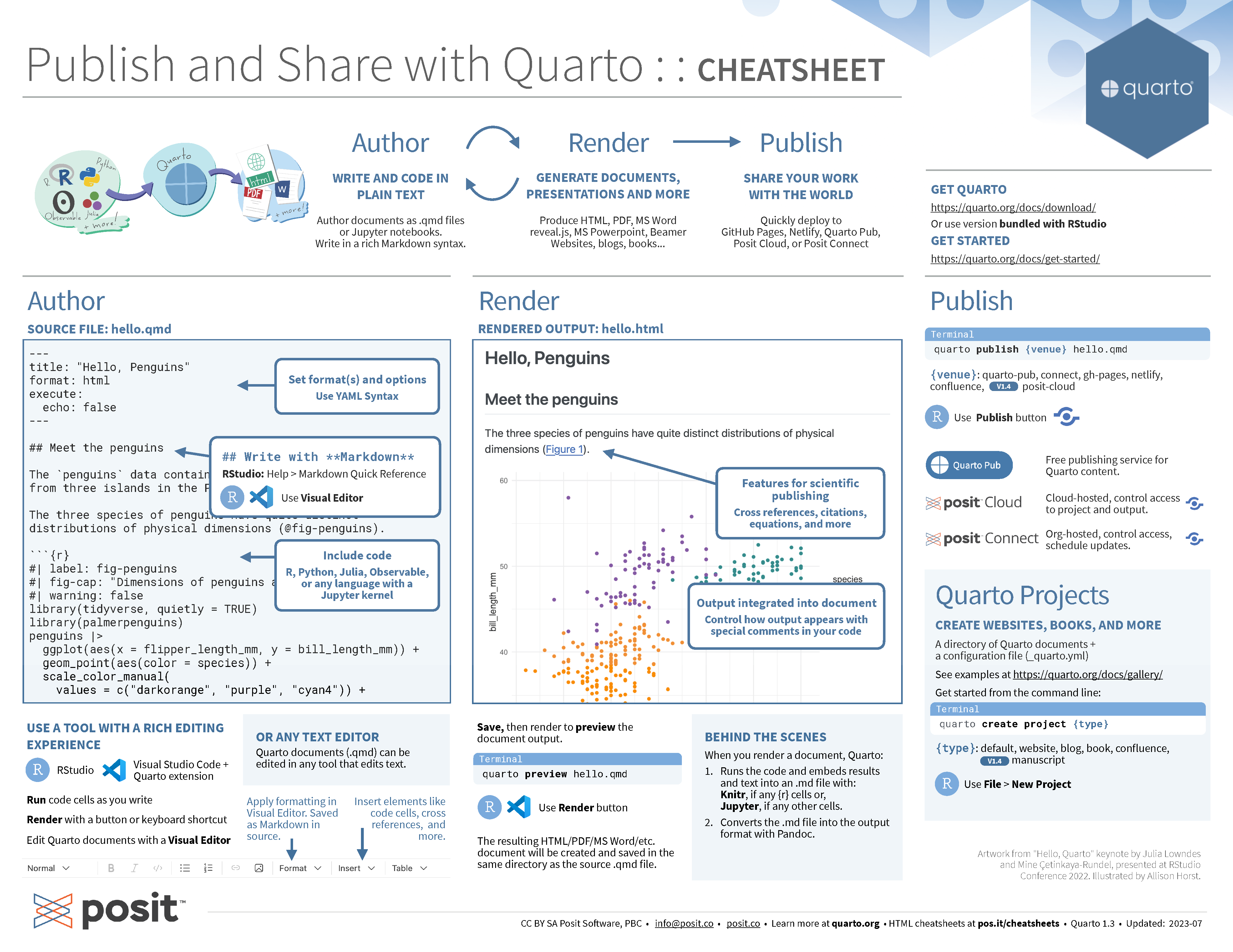
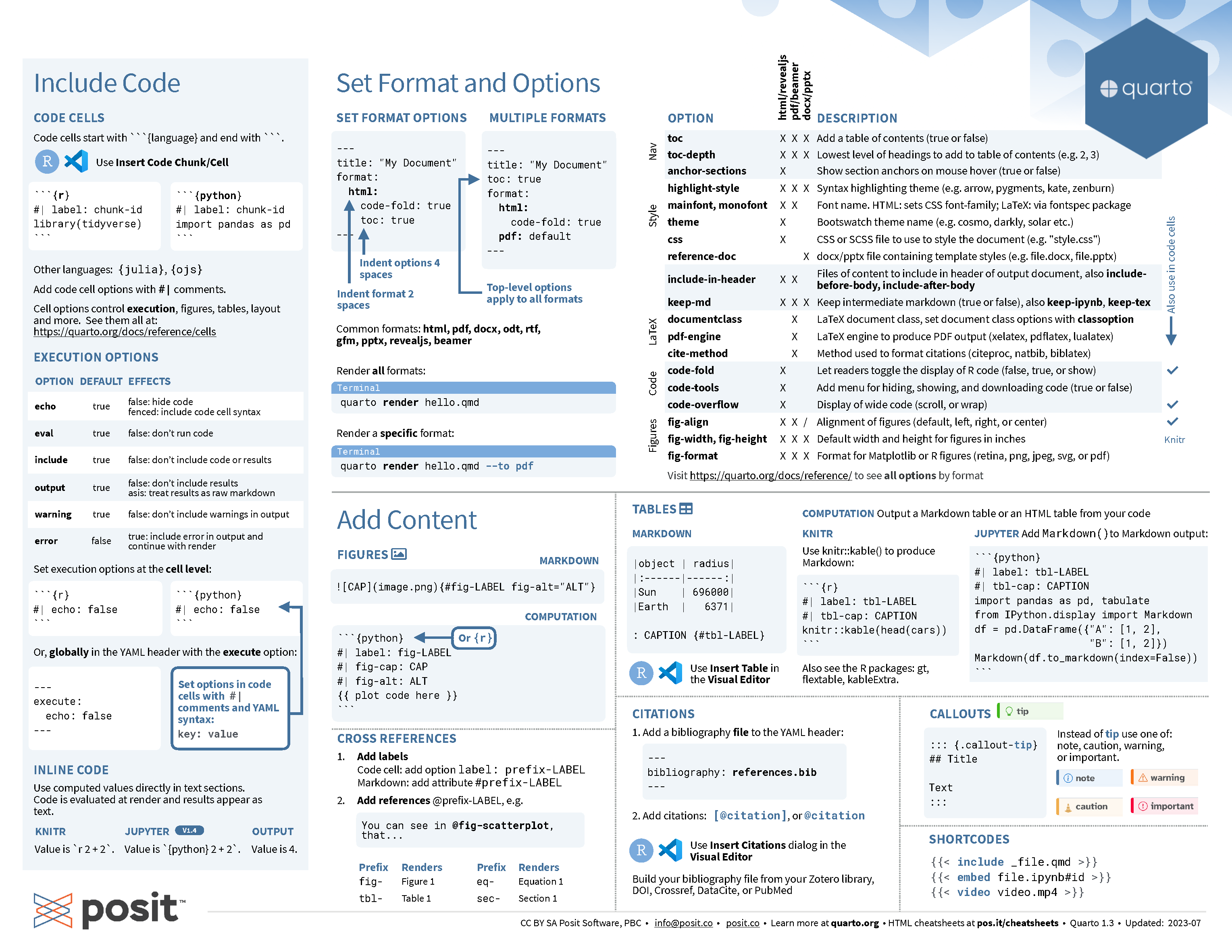
Quarto cheatsheet

Quarto cheatsheet

Literate Programming

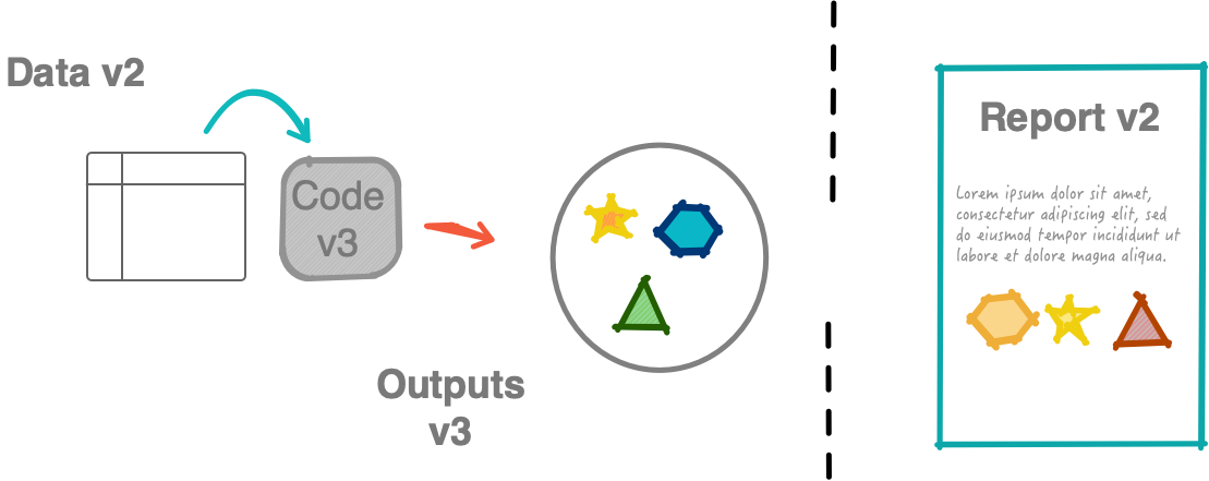
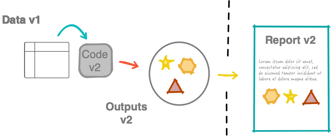
Non-robust workflow

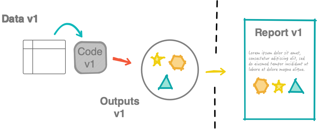
What should have been submitted:

A robust, reproducible workflow

• Using a robust, reproducible workflow means:
  • you avoid manual, repetitive tasks
  • your results are computationally reproducible
• Using a robust, reproducible workflow doesn’t mean you won’t make mistakes, but it will help you minimise mistakes.

Literate programming is a programming paradigm introduced by Donald Knuth where it emphasises writing code for humans (i.e. intertwine code with natural language explanations).

• Literate programming includes documentation (detailed explanations, comments and annotations to provide context, rationale and insight into the program’s design and functionality).

Analysis framework

Tidy data

1. Each column is a variable.
2. Each row is an observation.
3. Each cell is a single value.

Tools

• Git/GitHub for version control and collaboration
• Open-source programming languages (e.g. R and Python) for coding
• Quarto with markdown syntax for interoperable reproducible reports

• Huebner et al (2016) A systematic approach to initial data analysis is good research practice.
  The Journal of Thoracic and Cardiovascular Surgery
• Huebner et al (2018) A Contemporary Conceptual Framework for Initial Data Analysis. Observational Studies
• Steegen et al (2016) Increasing Transparency Through a Multiverse Analysis. Perspect Psychol Sci
• van der Loo & de Jonge (2018) Statistical Data Cleaning with Applications in R.
• Wickham (2014) Tidy Data. Journal of Statistical Software

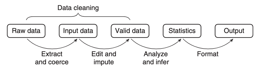
Statistical value chain

… a statistical value chain is constructed by defining a number of meaningful intermediate data products, for which a chosen set of quality attributes are well described …

– van der Loo & de Jonge (2018)

Schema from Mark van der Loo and Edwin de Jonge. 2018. Statistical Data Cleaning with Applications in R. John Wiley and Sons Ltd.

Folder structure

A suggested folder structure for data projects:

    project-root-folder/  # Root of the project folder
    │
    ├── README.md         # README file
    │
    ├── data/             # Raw and derived data
    │   ├── data-raw/     # Read-only files
    │   ├── data-input/   # Extracted and coerced from raw data
    │   ├── data-valid/   # Edit and imputed from input data
    │   └── data-stats/   # Analysed results (R objects, .csv, etc.)
    │
    ├── analysis/         # Scripts (not functions) to run analysis
    │
    ├── figures/          # Figures (.png, .pdf, etc.)
    │
    ├── misc/             # Misc
    │
    ├── report.qmd        # Report, paper, or thesis output

Sharing your documents

via Quarto Pubs

• Make sure you are logged in to your Quarto Pub account.
• Then run the following command in the Terminal:

quarto publish quarto-pub /path/to/your/quarto-document.qmd

Self-contained HTML document

format:
  html:
    embed-resources: true

then you can share your output HTML file with no external dependencies

Happy writing and sharing 😊