Human brain
- Our brains can dissect and process features of images, e.g. the shape, object, lighting, etc.
- The human brain is made of billions of neurons that communicate via electrochemical signals.
- So how do we mimic this in a program?
Biological neuron model
- Artificial neural network, or often referred to just as neural network, was inspired by the biological neural network.
- In a biological neural network, a collection of neurons interconnected by synapses carry out a specific function when activated.
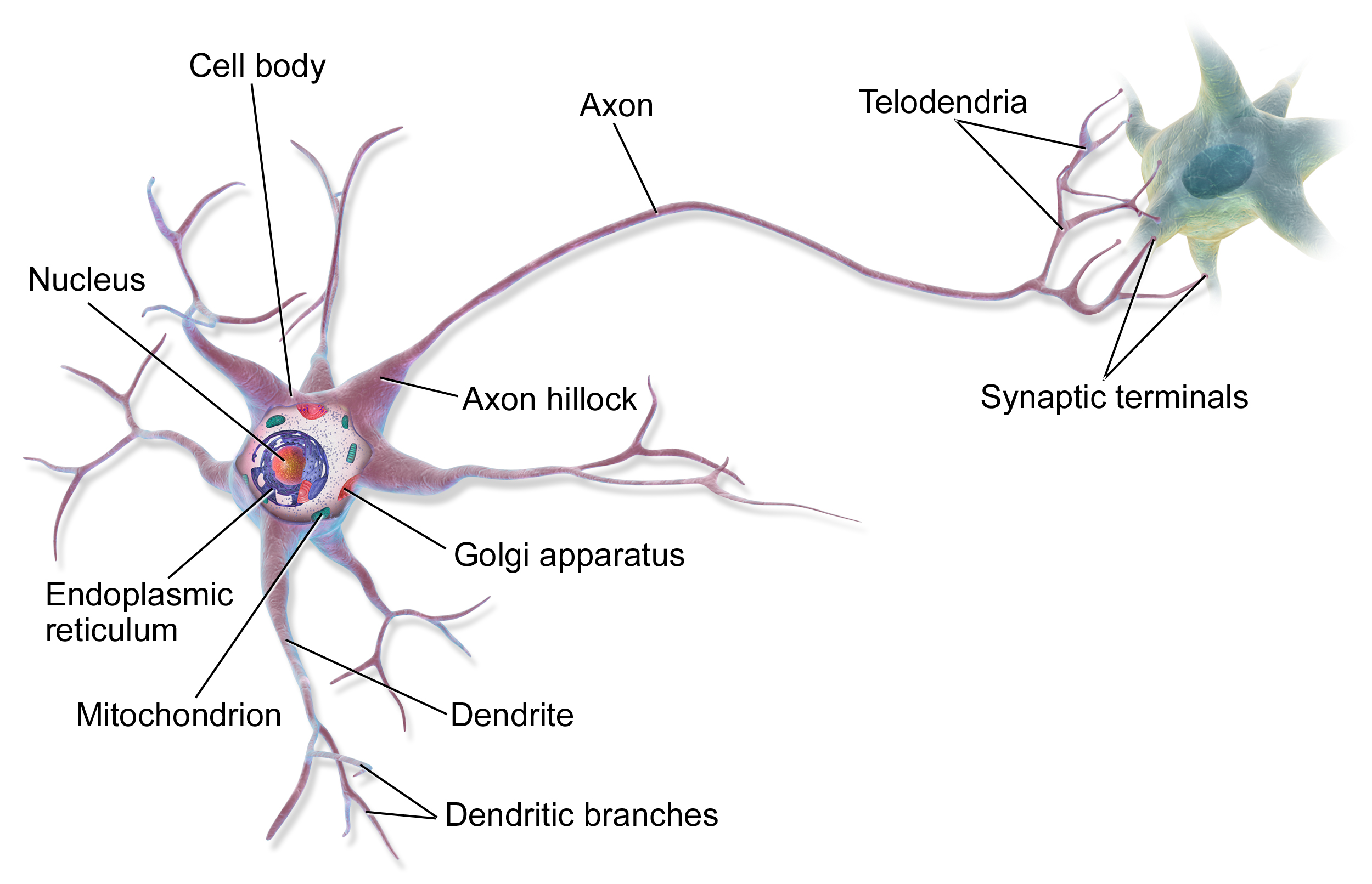
- The dendrites receive synaptic inputs and propogate electrochemical stimulation to the cell body - if stimulated enough, a neuron fires an action potential (synaptic inputs for other neurons).
Artificial neuron: dendrites
- The artificial neuron is the elementary units of an artificial neural network.
- The artificial neuron receives predictors \boldsymbol{x}_i = (1, x_{i1}, \dots,x_{ip})^\top that is typically combined as a weighted sum:

z_i = \beta_0 + \sum_{j=1}^p\beta_jx_{ij} = \boldsymbol{\beta}^\top\boldsymbol{x}_i, \quad\text{where }\boldsymbol{\beta} = (\beta_0, \beta_1, \dots, \beta_p)^\top.
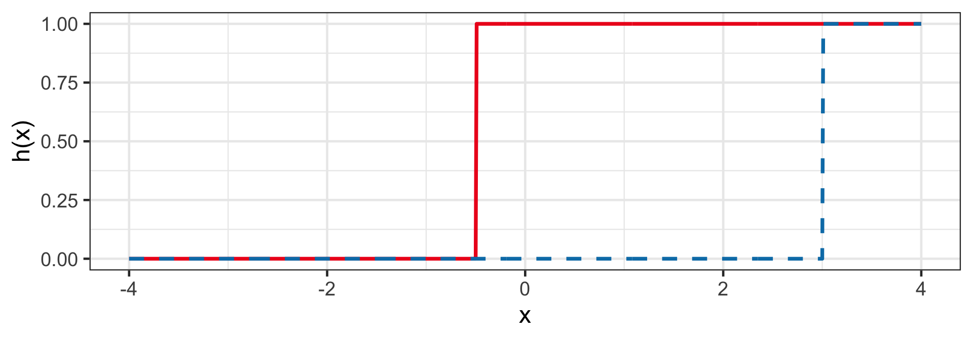
Heaviside step
h(z_i) = \mathbb{I}(z_i > 0)
- This is also known as the perceptron and is used for classification.
- For example: h(1 + 2x_i) and h(-12 + 4x_i).
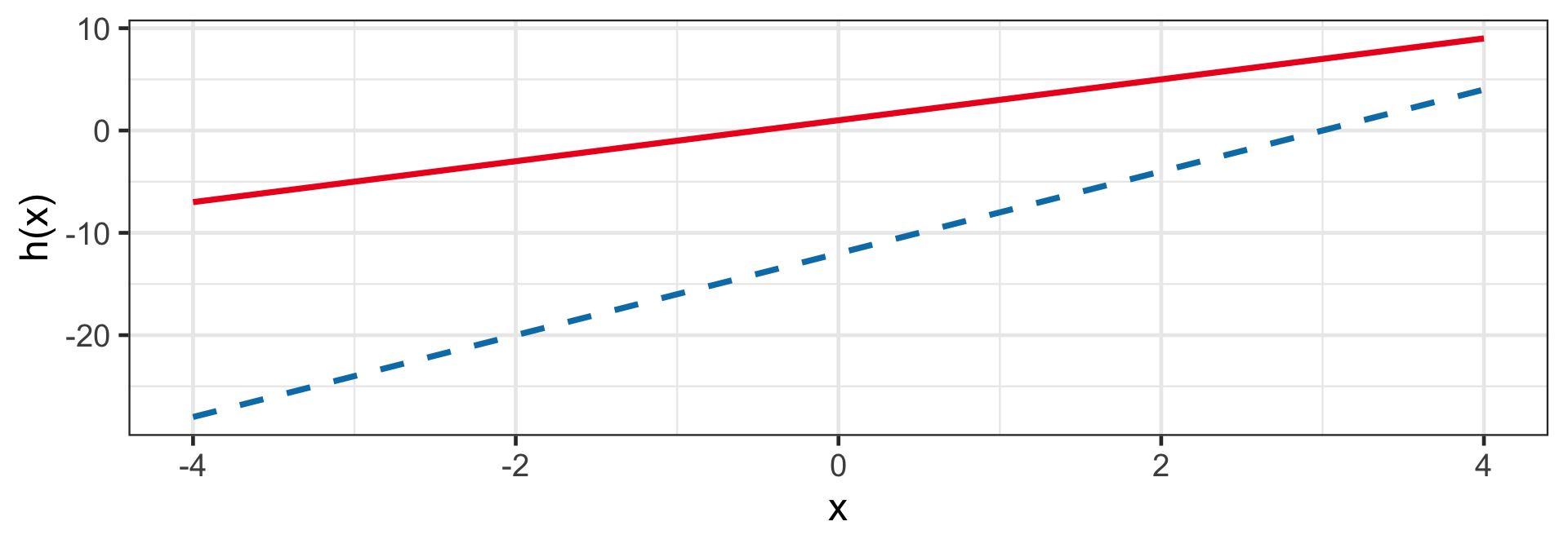
Linear
h(z_i) = z_i
- This is a regression model!
- For example: h(1 + 2x_i) and h(-12 + 4x_i).
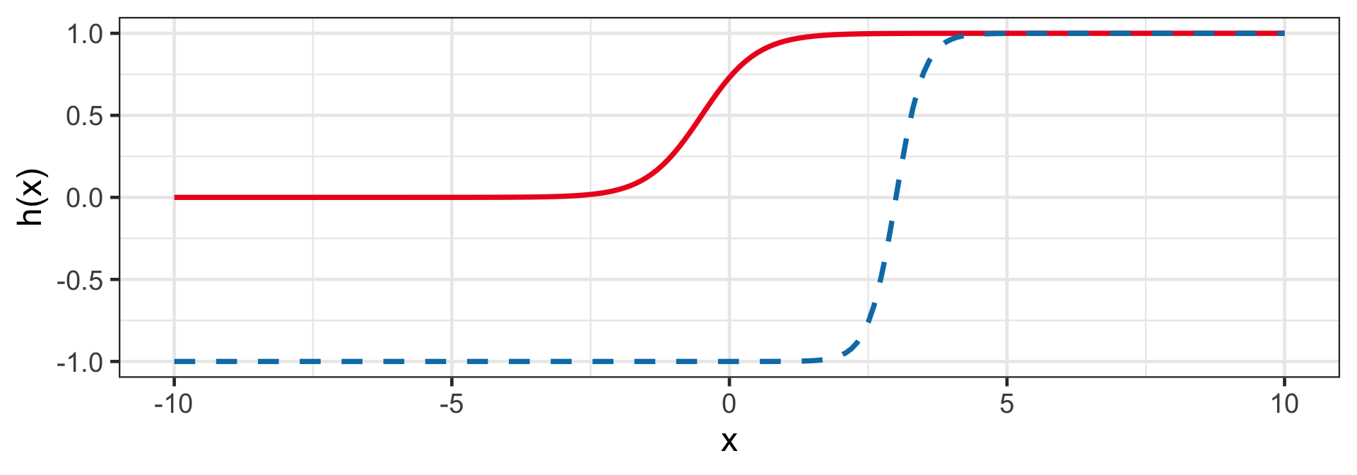
Sigmoid (Logistic)
h(z_i|a,w) = a + w(1+e^{-z_i})^{-1}
- When a = 0 and w = 1, then 0 < h(z_i) < 1 for finite z_i.
- E.g. h(1 + 2x_i|a = 0, w = 1) and h(-12 + 4x_i|a = -1, w = 2).
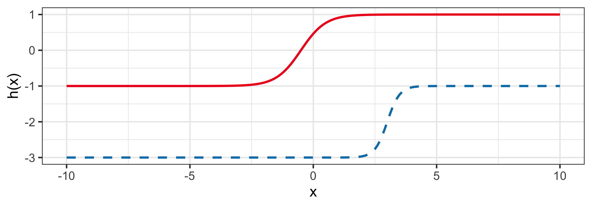
Hyperbolic tangent (Tanh)
h(z_i) = a + w \left(\frac{2}{1+e^{-2z_i}} - 1 \right)
- Similar to Sigmoid.
- E.g. h(1 + 2x_i|a = 0, w = 1) and h(-12 + 4x_i|a = -1, w = 2).
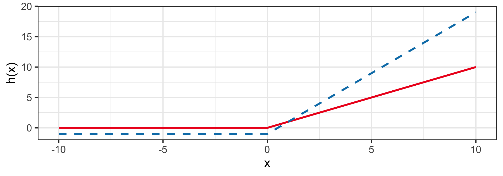
Rectified linear unit (ReLU)
h(z_i) = a + w \times \max(0, z_i)
- Sigmoid and Tanh are largely replaced by rectified linear unit (ReLU).
- E.g. h(1 + 2x_i|a = 0, w = 1) and h(-12 + 4x_i|a = -1, w = 2).
Takeaways
- Neural networks are flexible models that can be used for both regression and classification problems.
- The activation function in the output layer determine if the neural network can be used for regression or classification.
- More neural network to come next week!