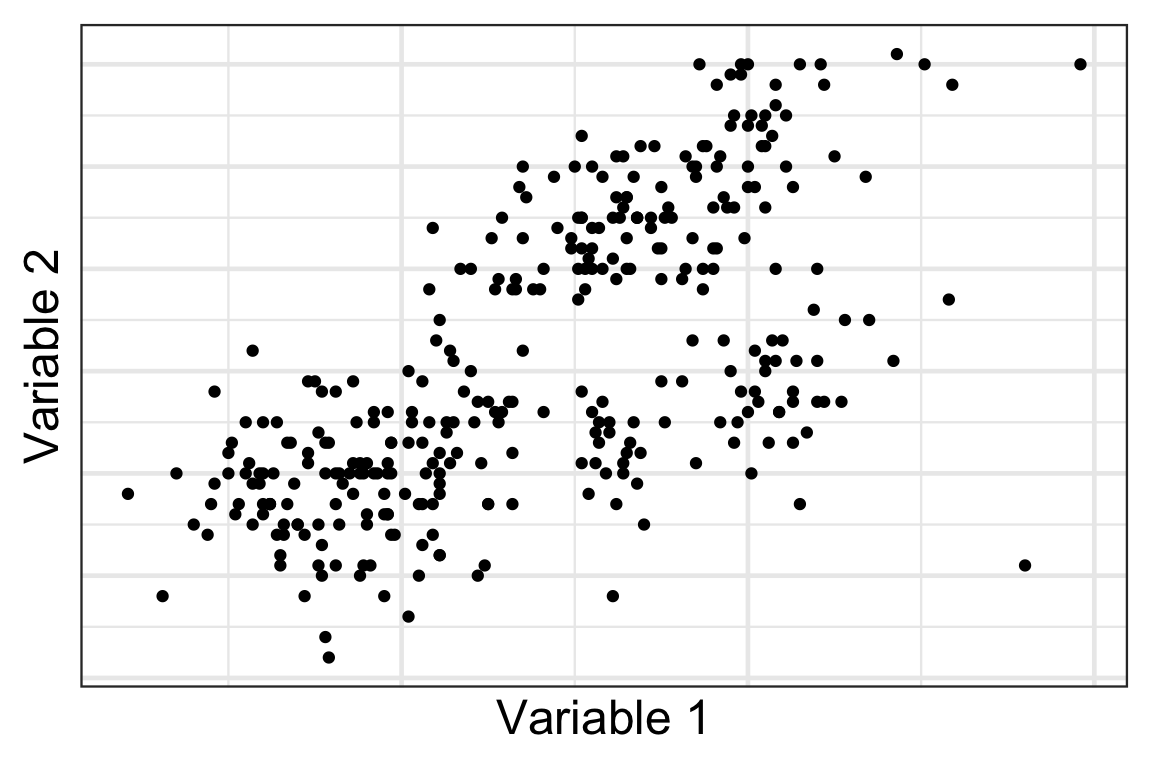
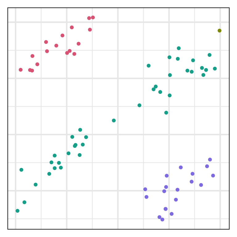
A possible clustering
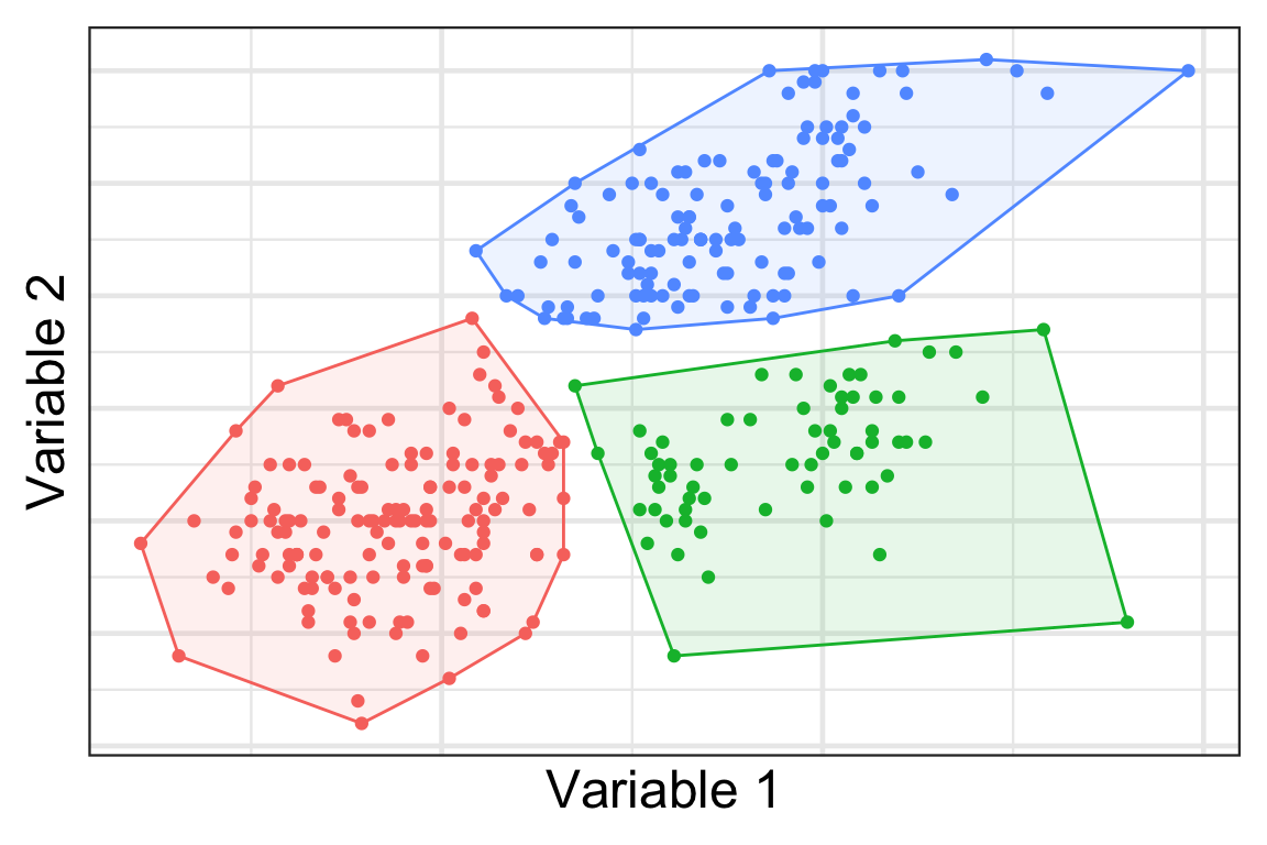
- Here we cluster the observations into 3 groups… but how?
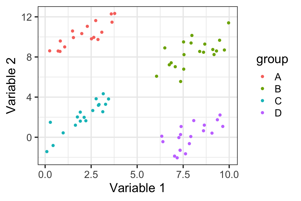
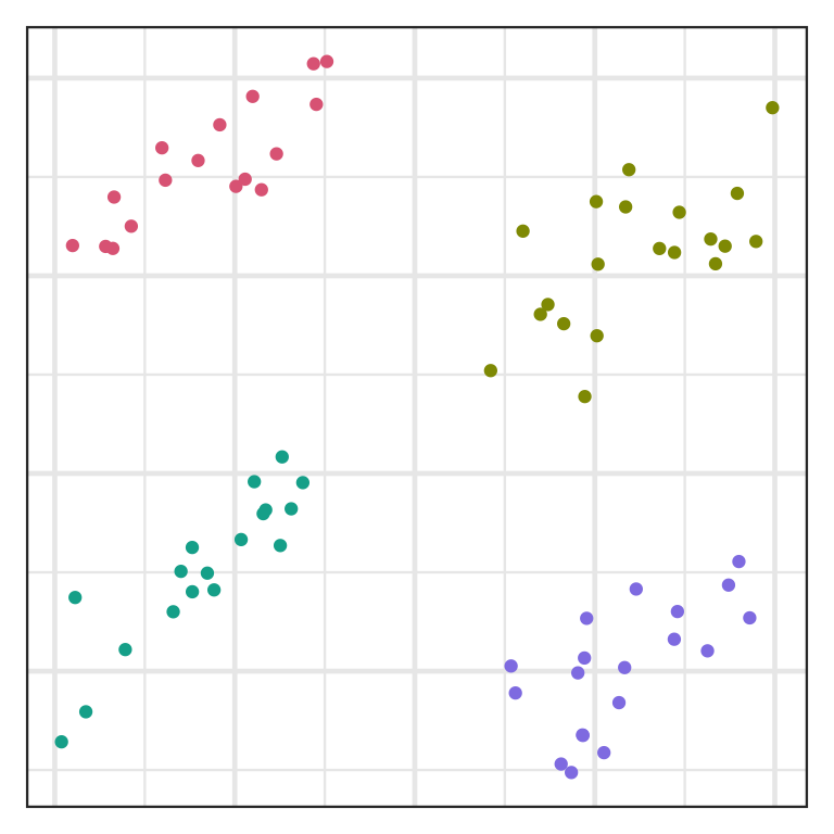
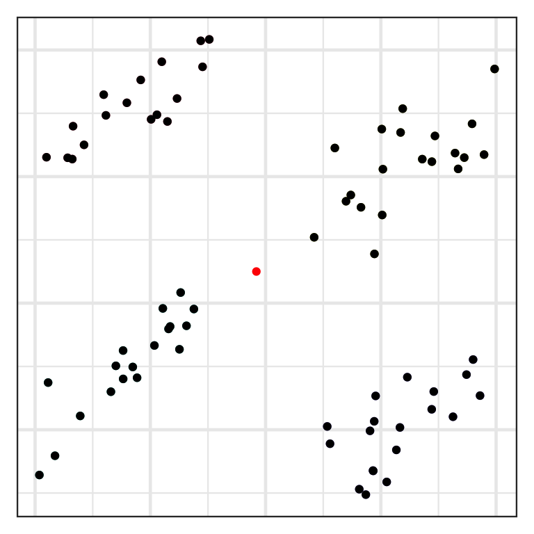
Toy data
- Suppose we have this data with four groups shown below.
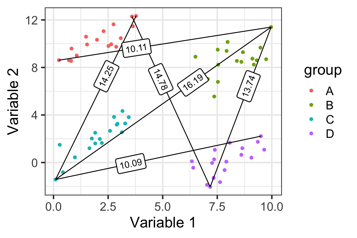
Single linkage
D(\mathcal{A}, \mathcal{B}) = \min_{i\in\mathcal{A},j\in\mathcal{B}}D(\boldsymbol{x}_i,\boldsymbol{x}_j)
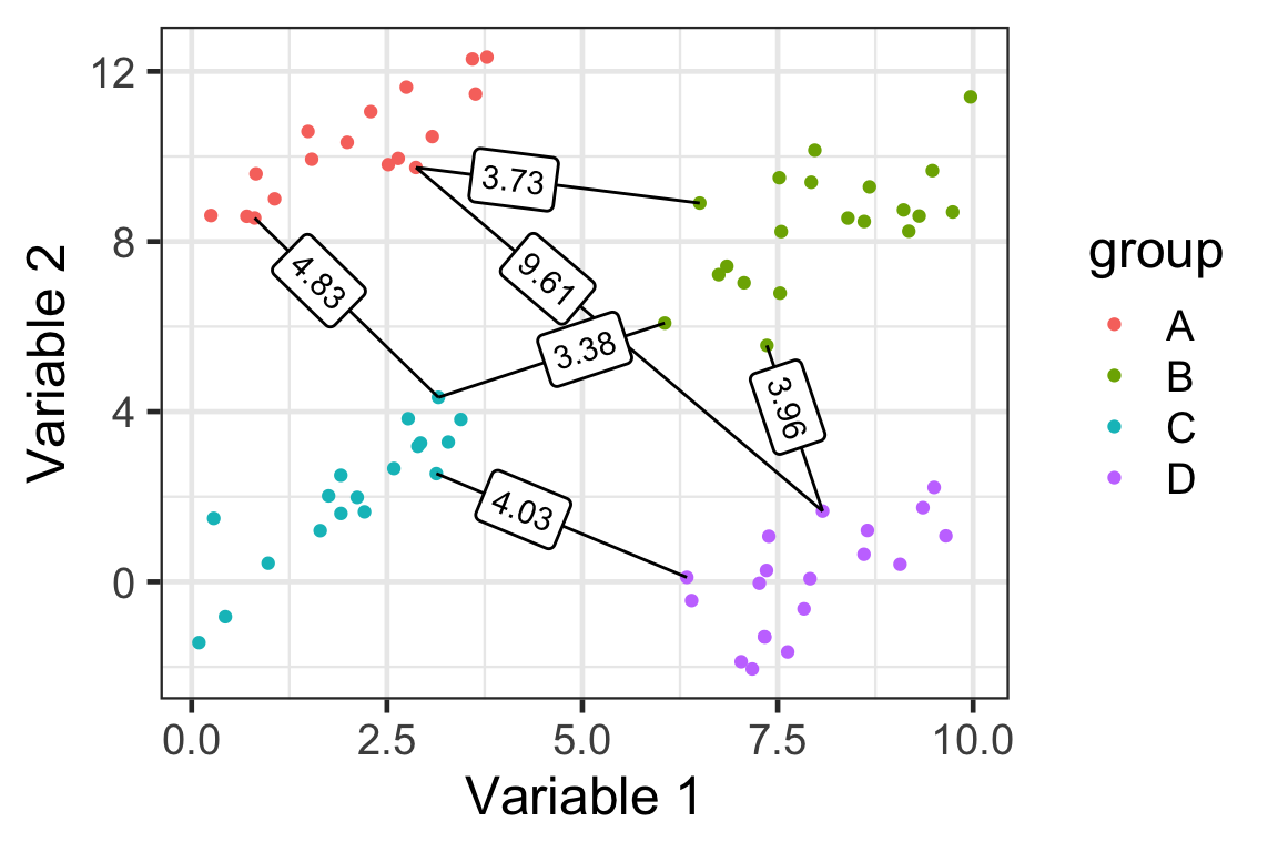
- Here we have 4 groups and 6 distances (based on ED) between clusters.
Complete linkage
D(\mathcal{A}, \mathcal{B}) = \max_{i\in\mathcal{A},j\in\mathcal{B}}D(\boldsymbol{x}_i,\boldsymbol{x}_j)
Average linkage
D(\mathcal{A}, \mathcal{B}) = \frac{1}{|\mathcal{A}||\mathcal{B}|}\sum_{i\in\mathcal{A}}\sum_{j\in\mathcal{B}}D(\boldsymbol{x}_i,\boldsymbol{x}_j)

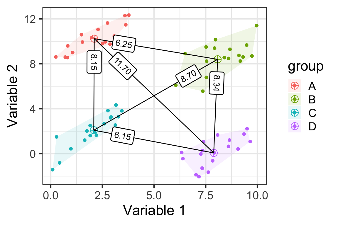
Centroid linkage
D(\mathcal{A}, \mathcal{B}) = D(\bar{\boldsymbol{x}}_\mathcal{A},\bar{\boldsymbol{x}}_\mathcal{B})
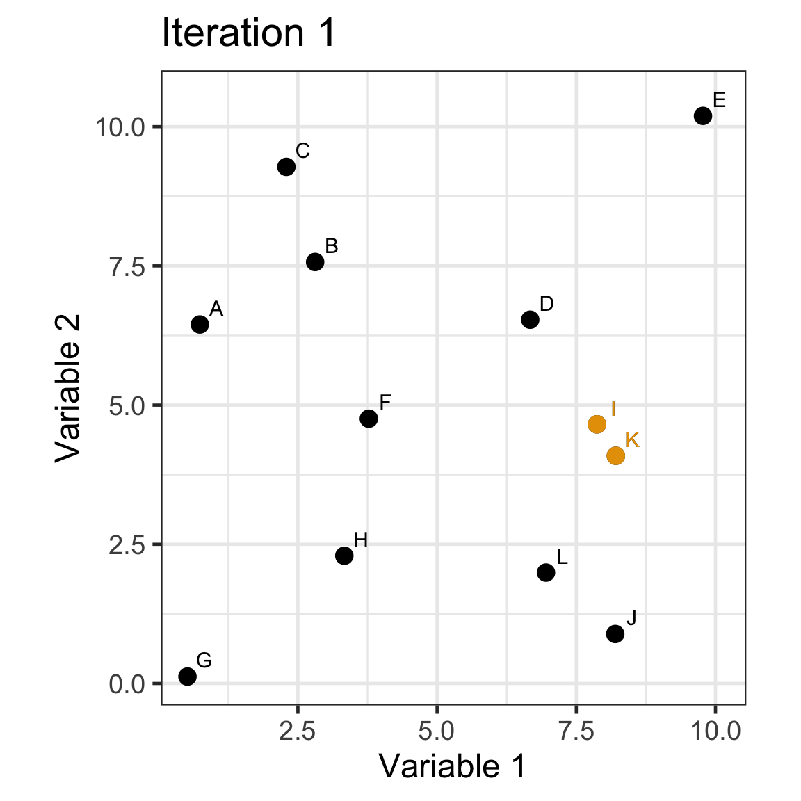
Single linkage demo: iteration 0
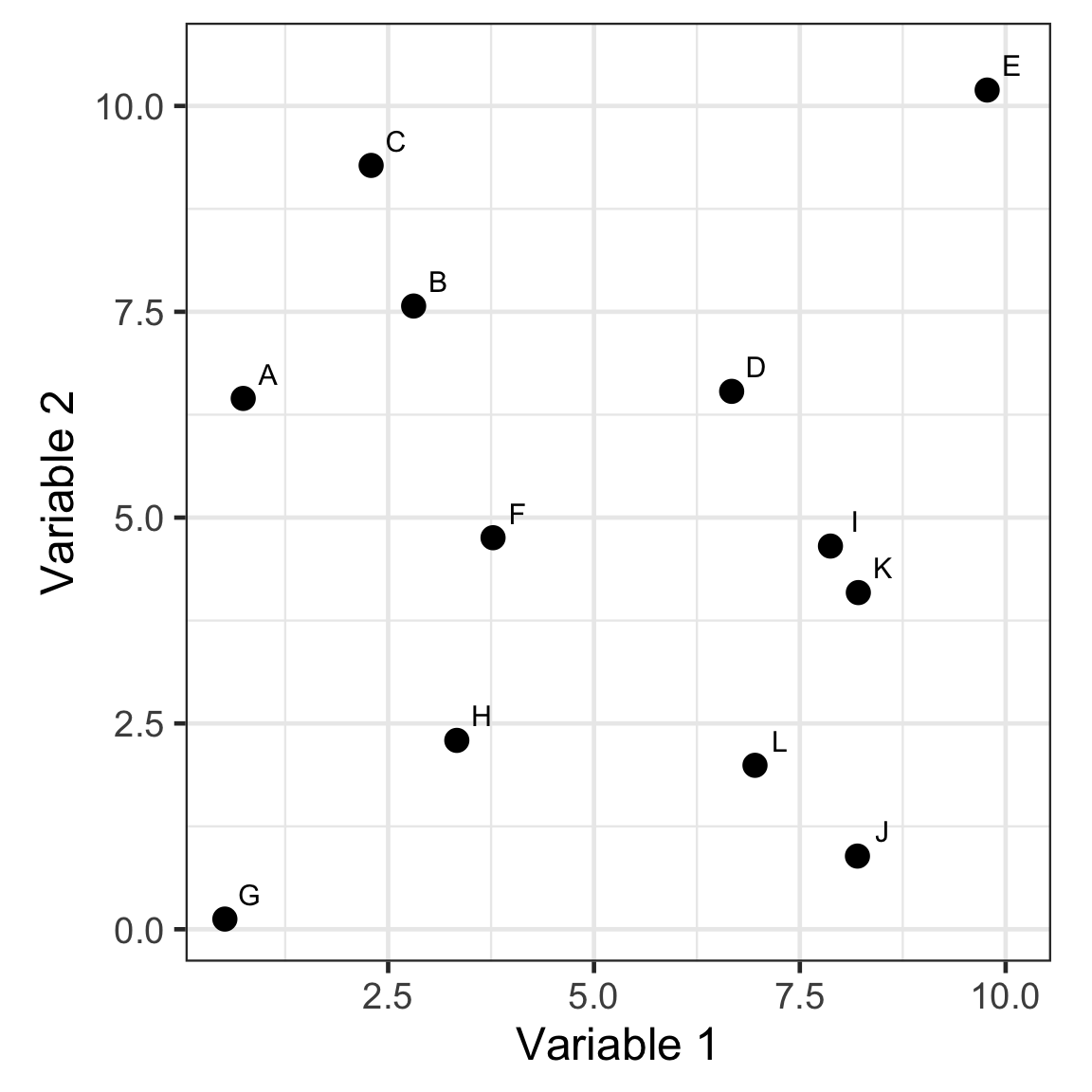
- Every observation starts as a singleton cluster.
Single linkage demo: iteration 1
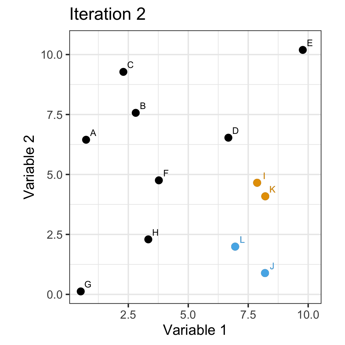
Single linkage demo: iteration 2
Single linkage demo: iteration 3
Single linkage demo: iteration 4
Single linkage demo: iteration 5

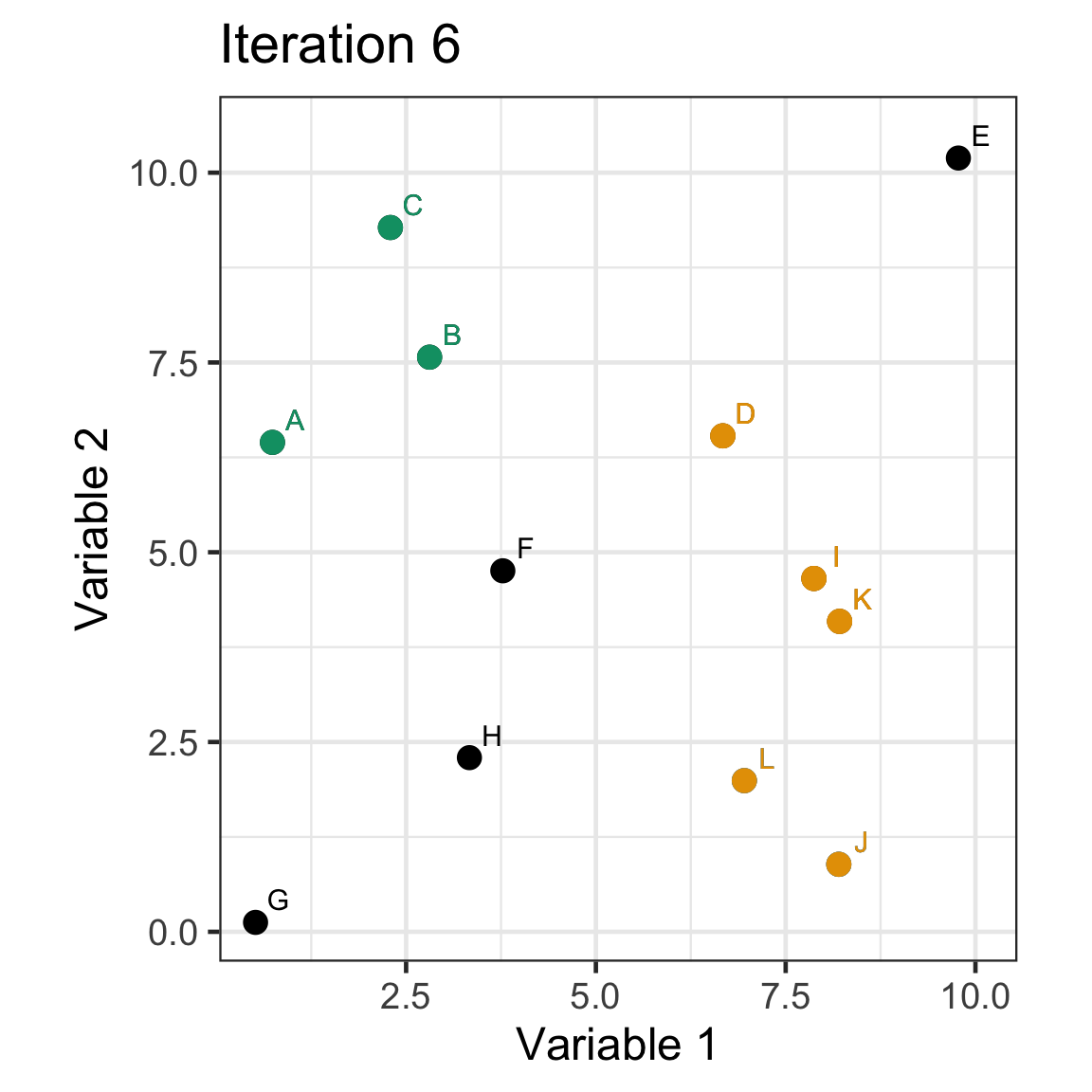
Single linkage demo: iteration 6
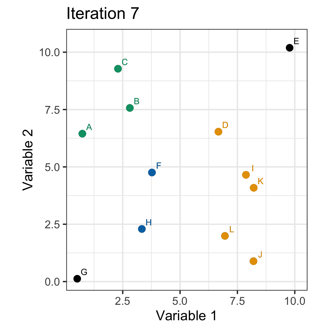
Single linkage demo: iteration 7
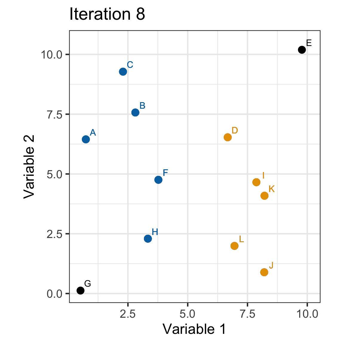
Single linkage demo: iteration 8
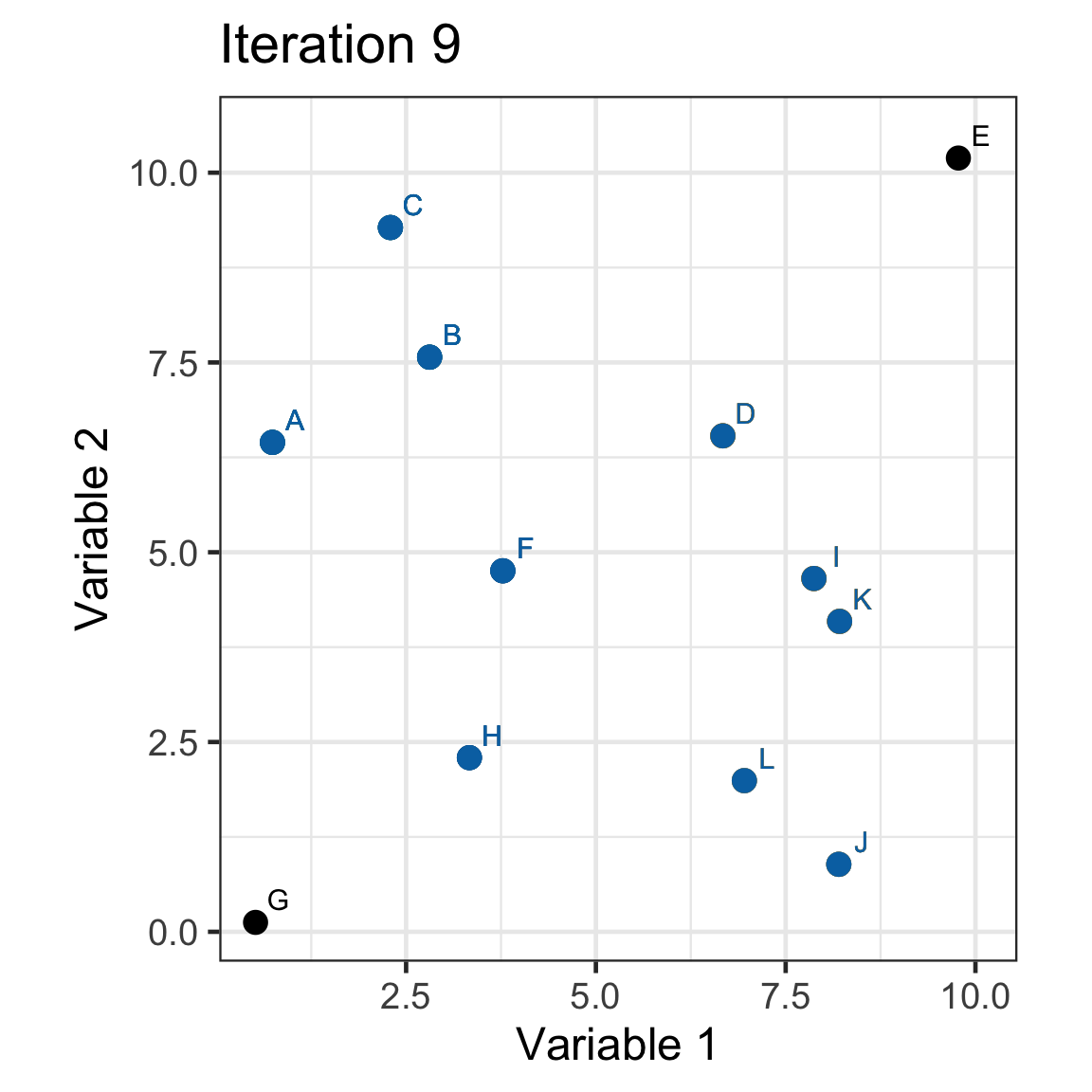
Single linkage demo: iteration 9
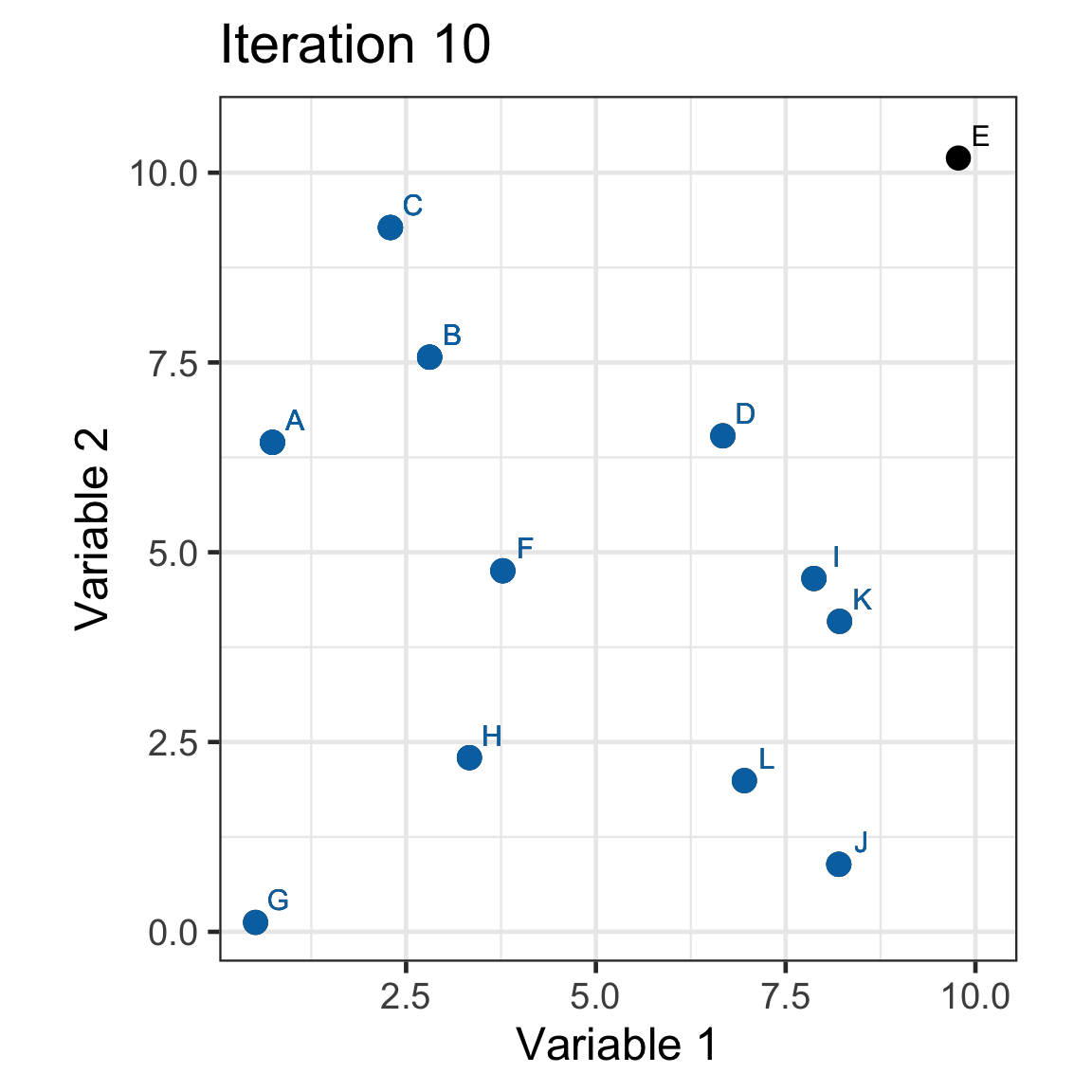
Single linkage demo: iteration 10
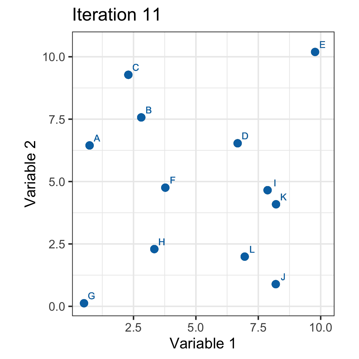
Single linkage demo: iteration 11
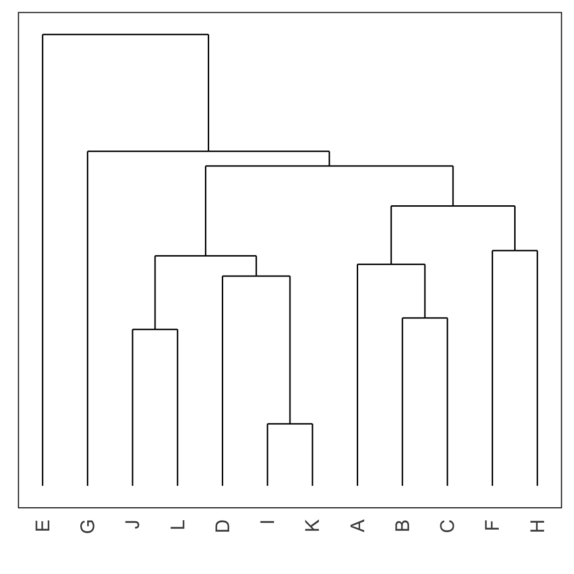
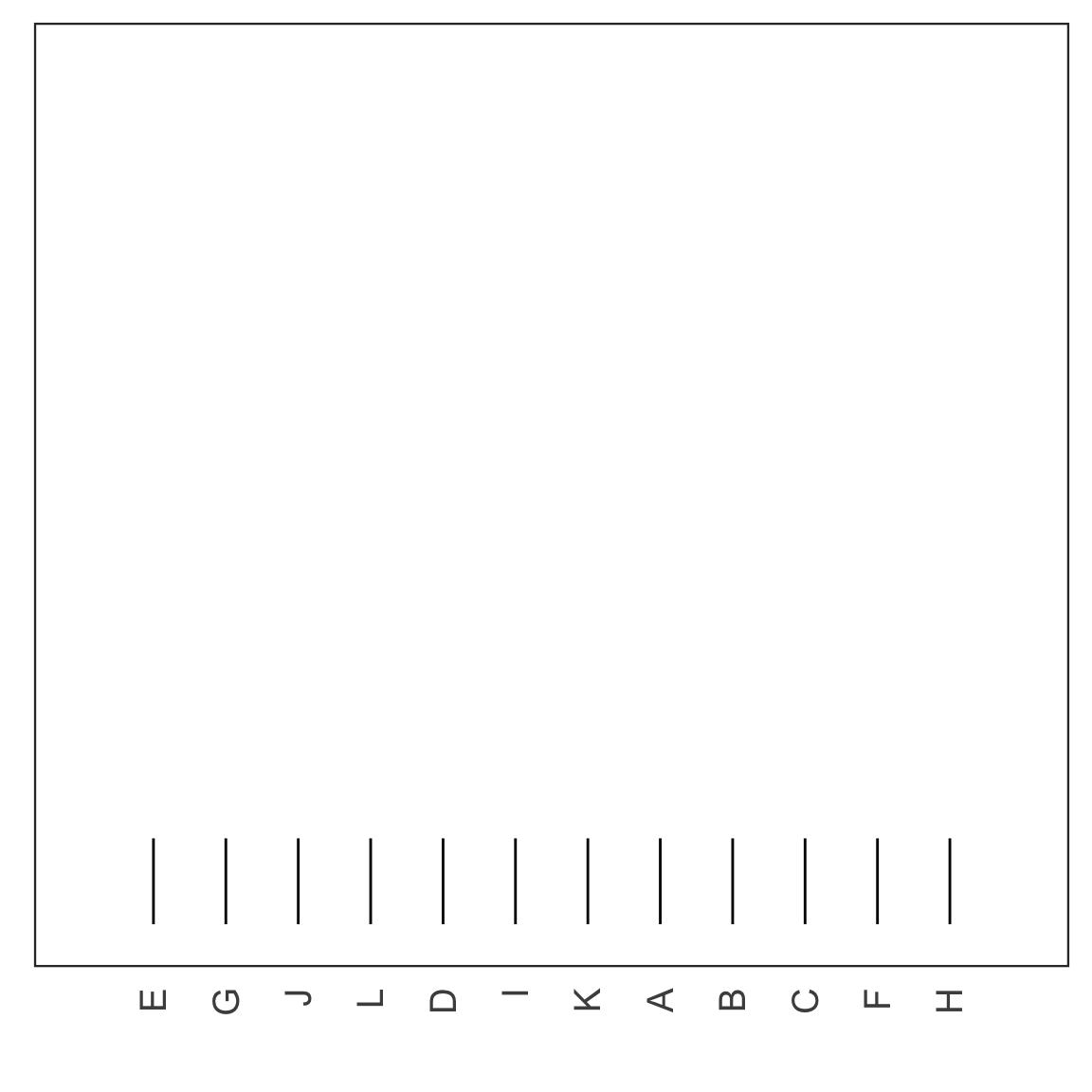
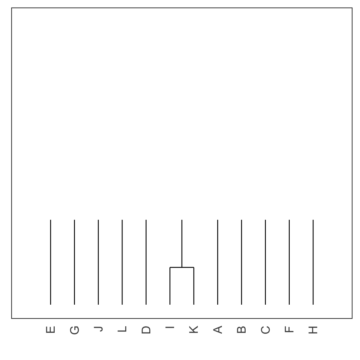
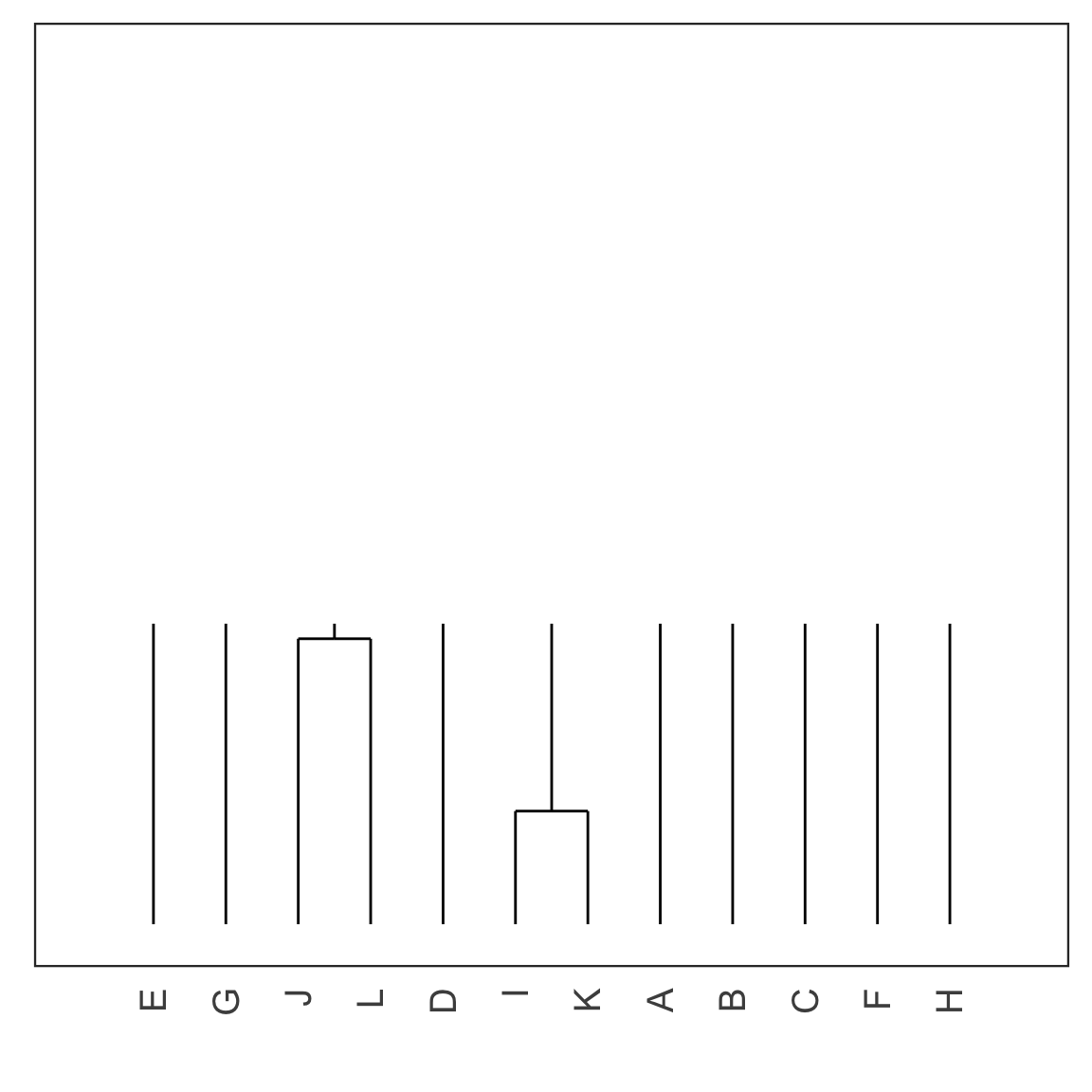
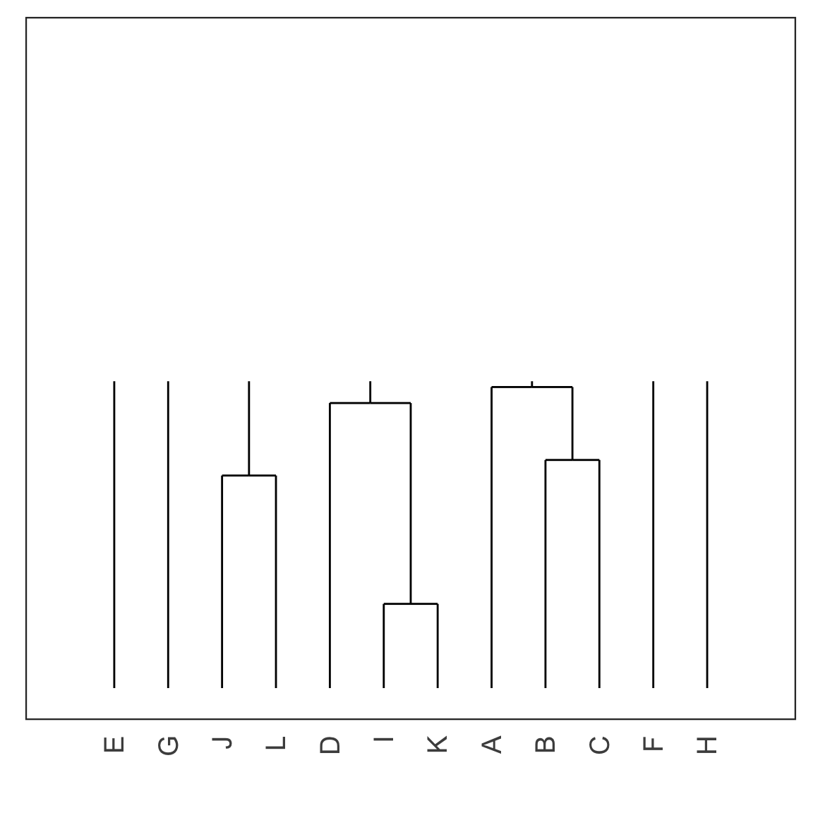
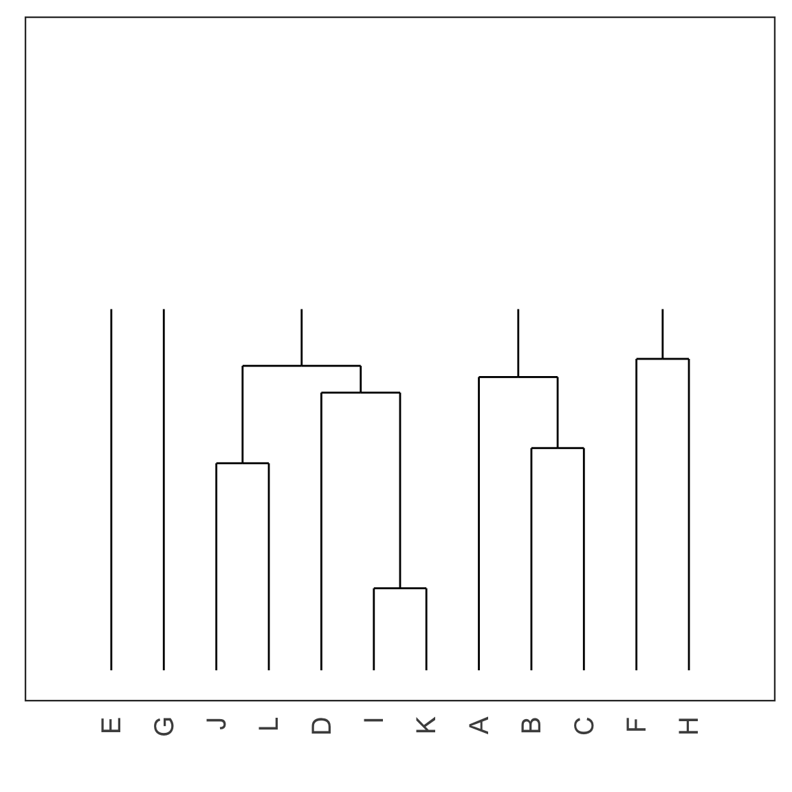
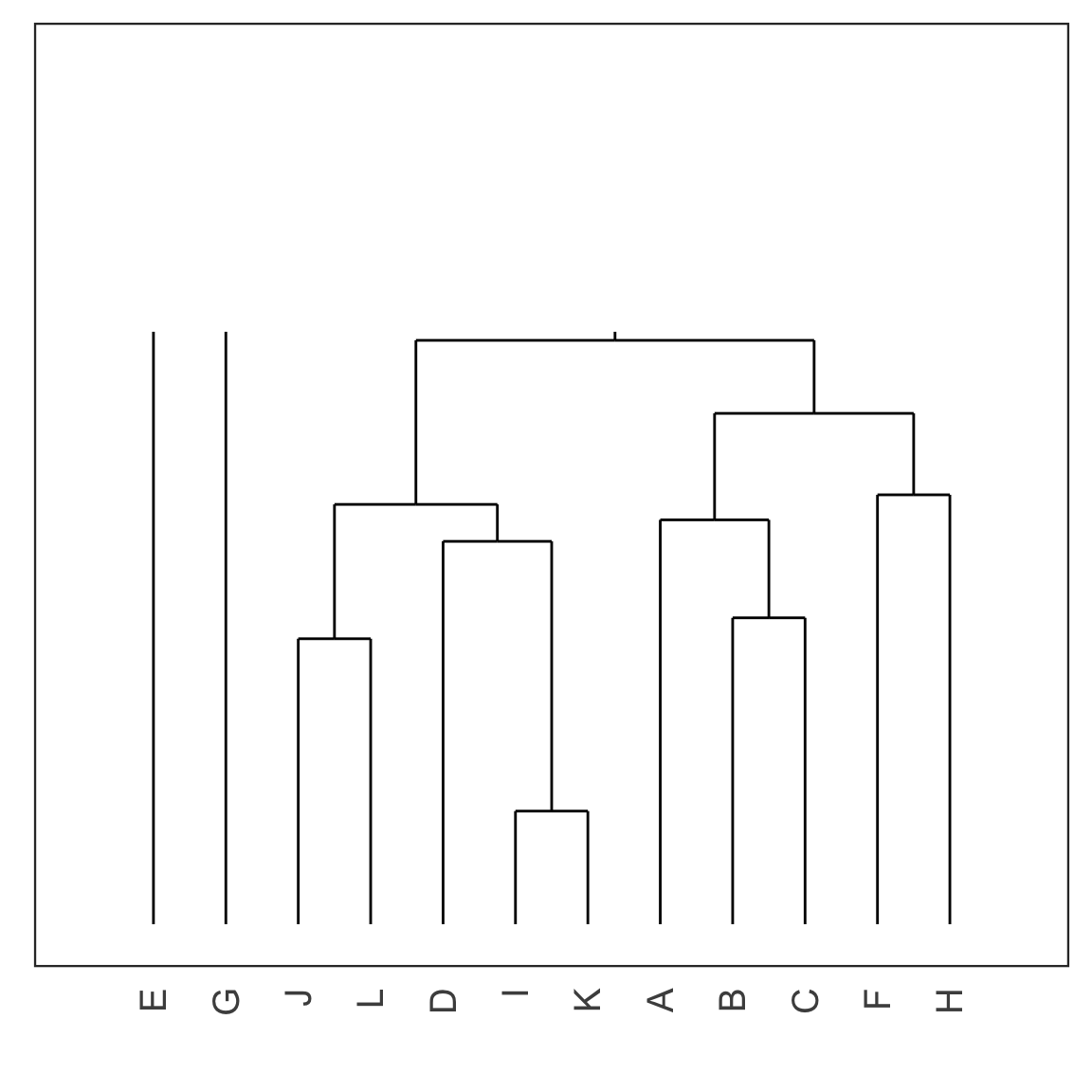
Dendrogram
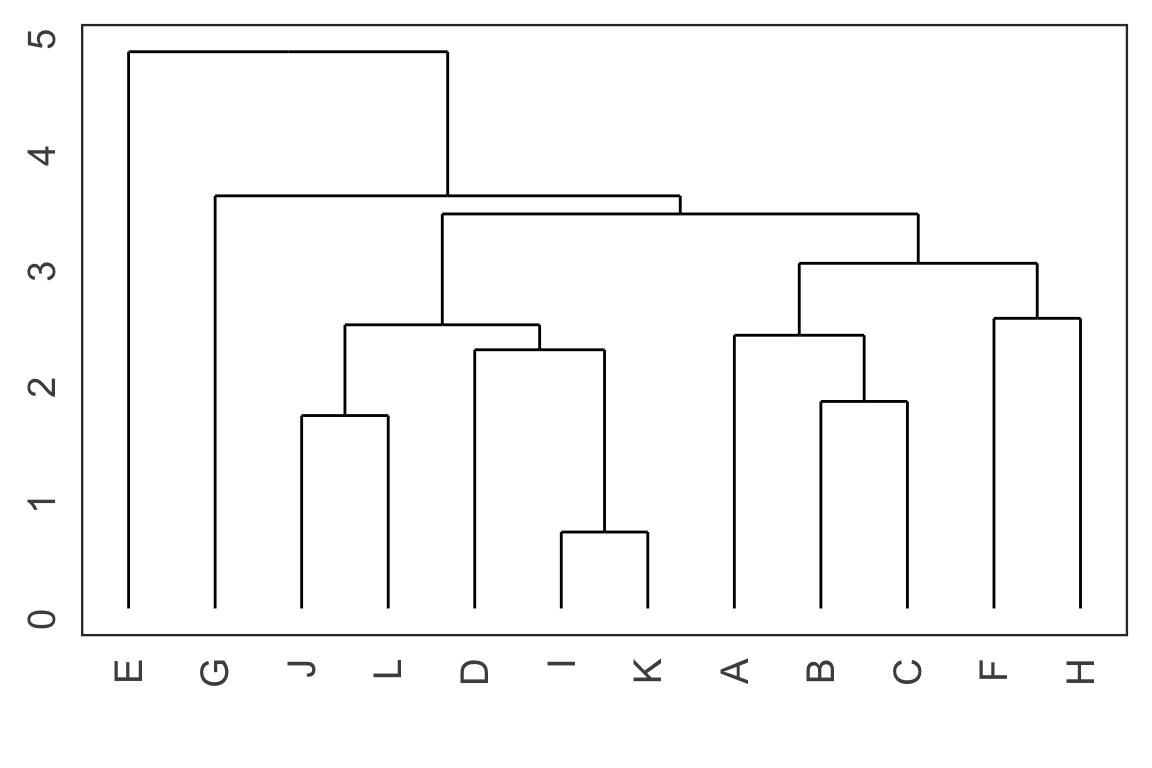
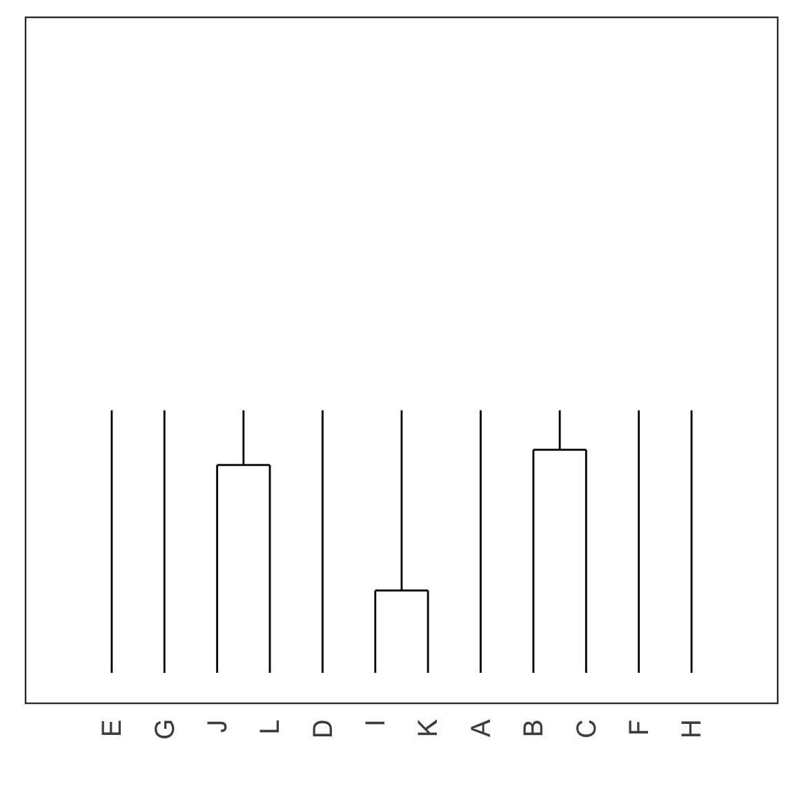
- Each leaf of the dendrogram represents one observation.
- Leaves fuse into branches and branches fuse, either with leaves or other branches.
- Fusions lower in the tree mean the groups of observations are more similar to each other.
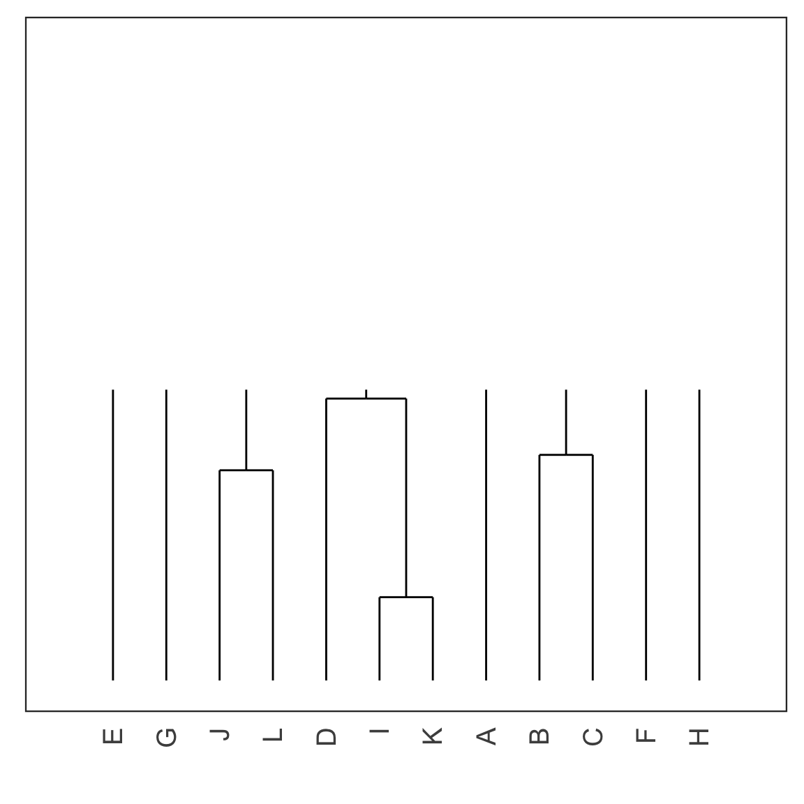
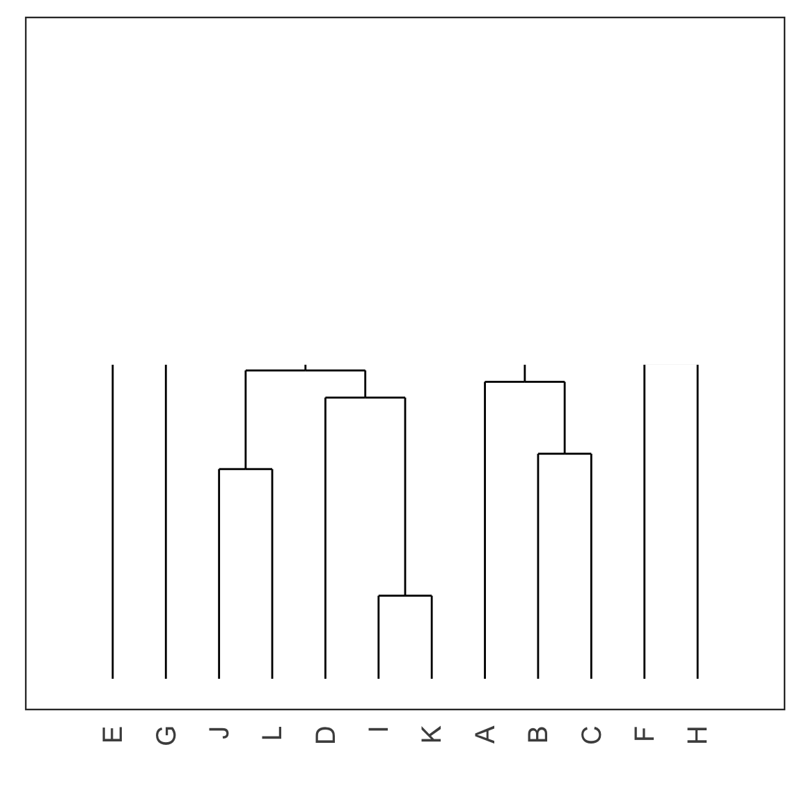
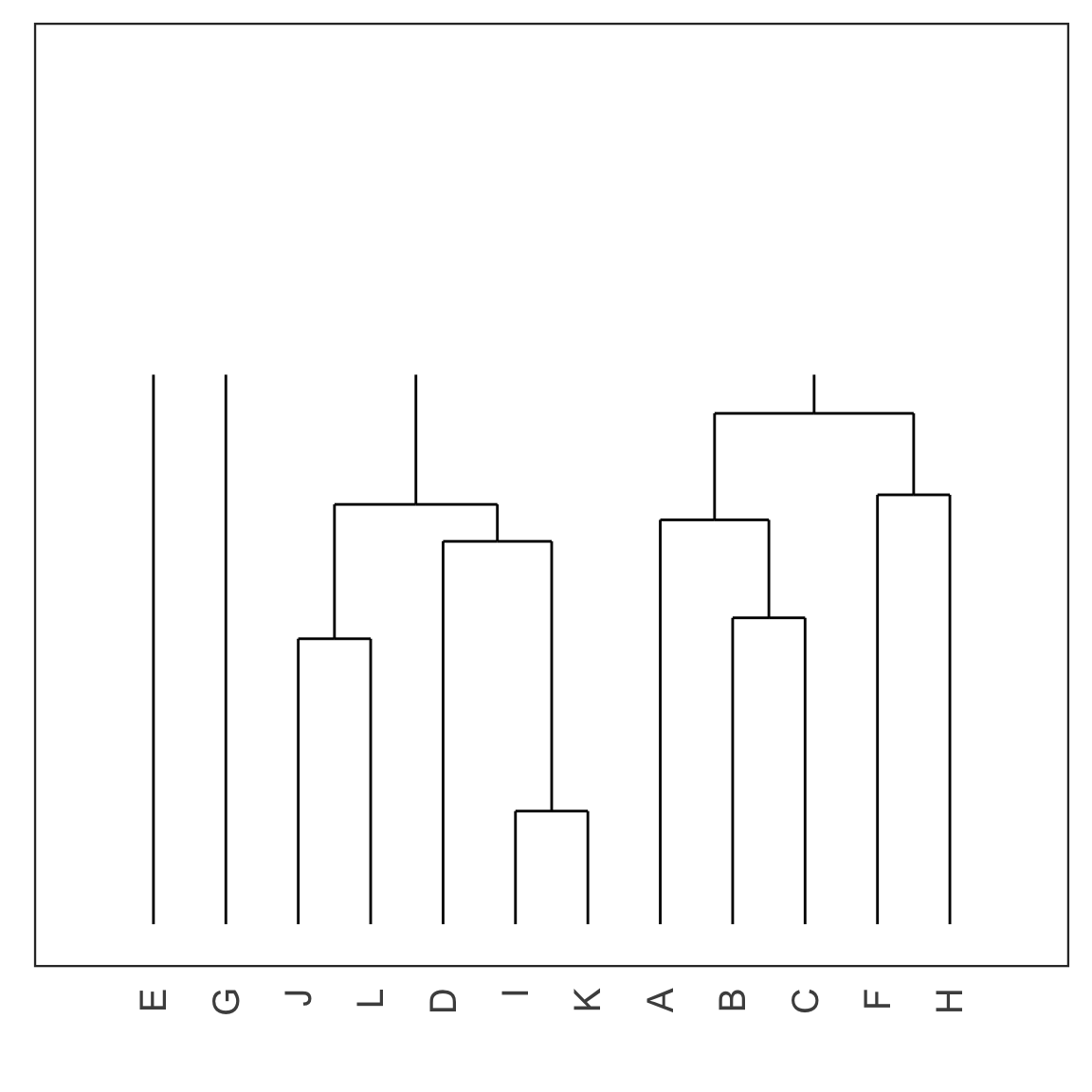
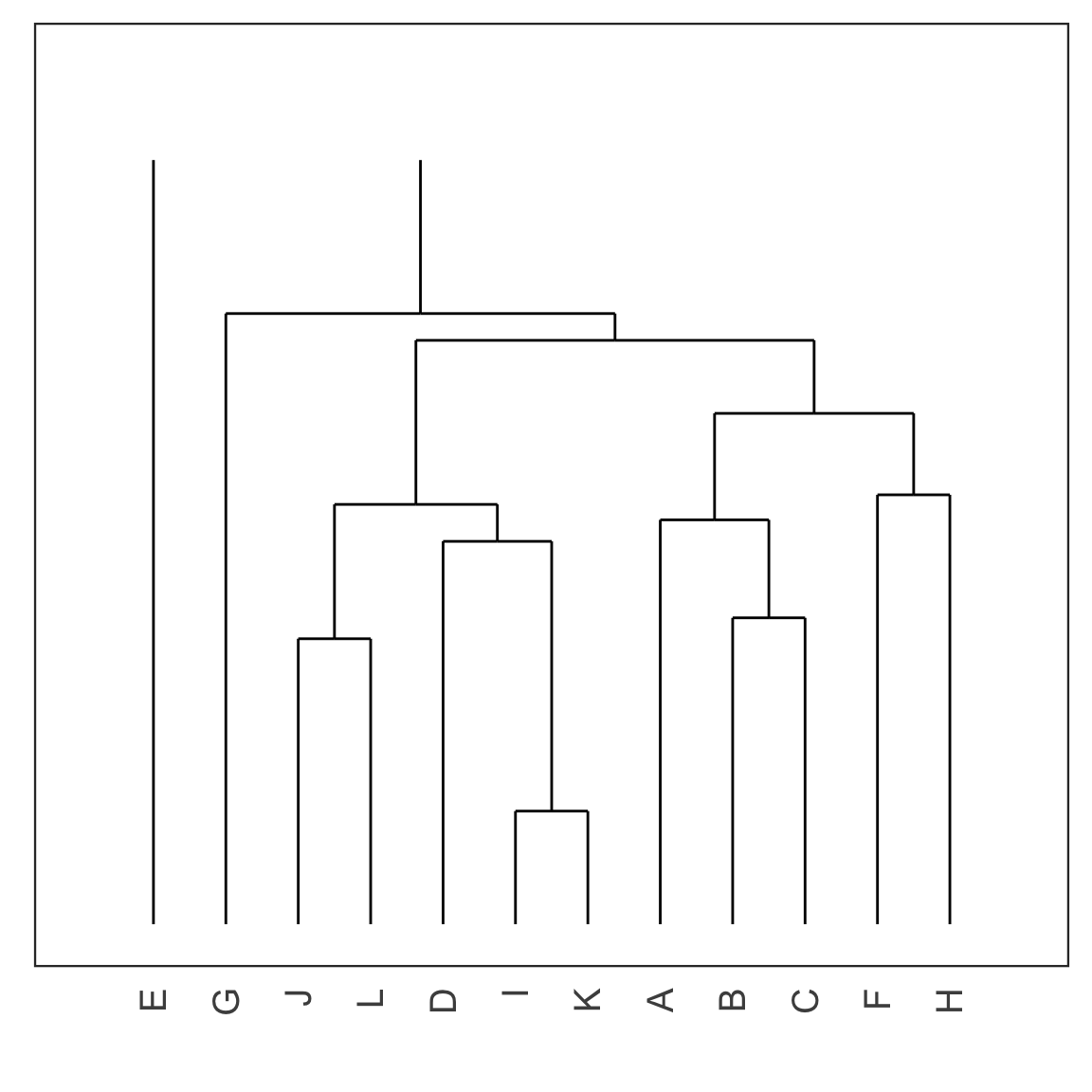
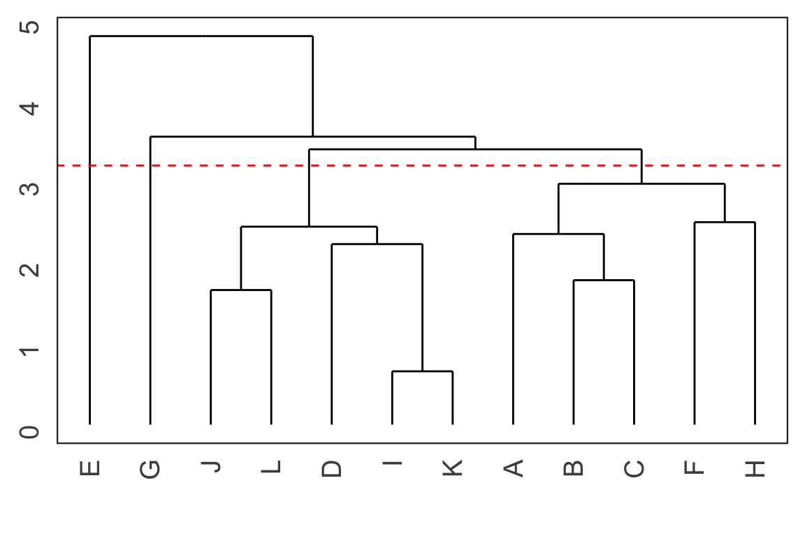
Cutting the tree
- Cut the tree at a particular height results in a particular set of clusters.
- For example, cutting the tree at the dashed red line below results in 4 clusters: (E), (G), (J, L, D, I K) and (A, B, C, F, H).
Chaining
- Single linkage often suffers from chaining, i.e. a single observation results in merging two clusters.
- This results in clusters that are spread out and not compact.
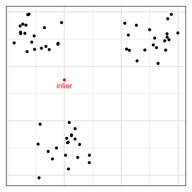
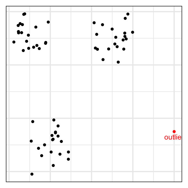
Inlier and outlier
- An inlier is an erroneous observation that lies within the interior of a distribution.
- An outlier is an observation that lies well outside the typical range of values.
Yale face database
Code
Sys.setenv(VROOM_CONNECTION_SIZE = 5000000)
yalefaces <- read_csv("https://emitanaka.org/iml/data/yalefaces.csv")

imagedata_to_plotdata <- function(data = yalefaces,
                                  w = 320,
                                  h = 243,
                                  which = sample(1:165, 15)) {
  data %>%
    mutate(id = 1:n()) %>%
    filter(id %in% which) %>%
    pivot_longer(starts_with("V")) %>%
    mutate(col = rep(rep(1:w, each = h), n_distinct(id)),
           row = rep(rep(1:h, times = w), n_distinct(id)))
}

gfaces <- imagedata_to_plotdata(yalefaces) %>%
    ggplot(aes(col, row)) +
    geom_tile(aes(fill = value)) +
    facet_wrap(~subject + type, nrow = 3) +
    scale_y_reverse() +
    theme_void(base_size = 18) +
    guides(fill = "none") +
    coord_equal()

gfaces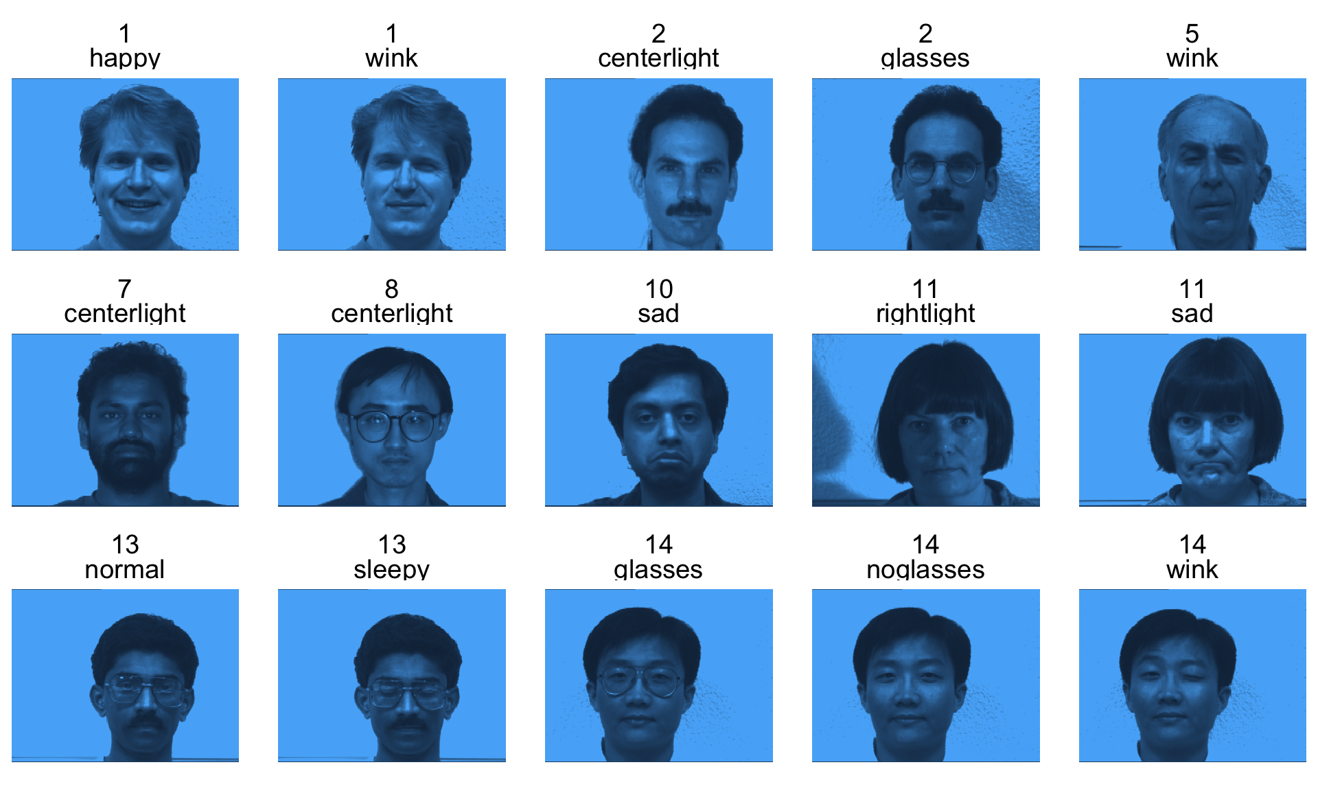
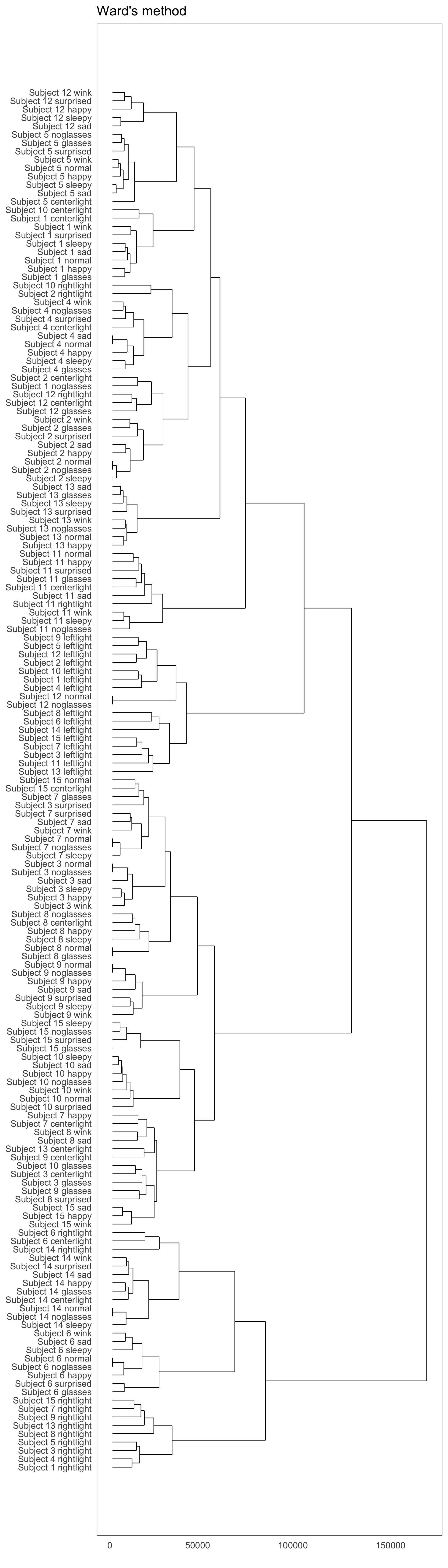
Dendrogram with R
scroll
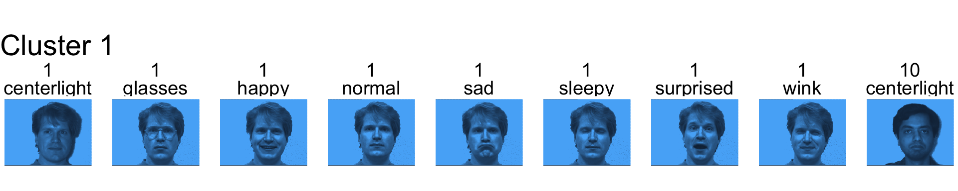
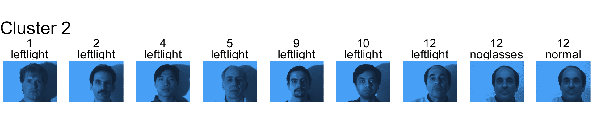
Clustering results
scroll
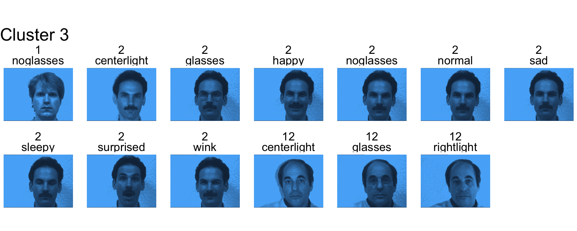
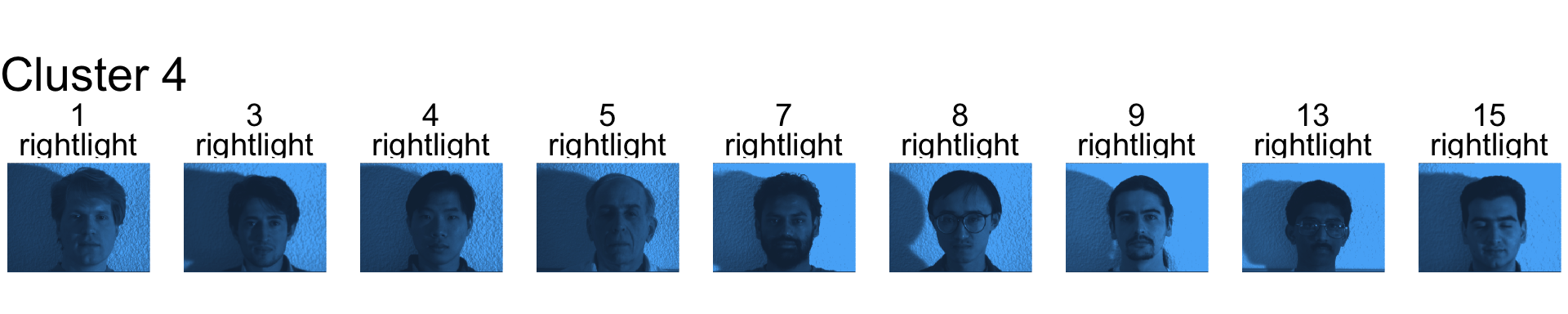
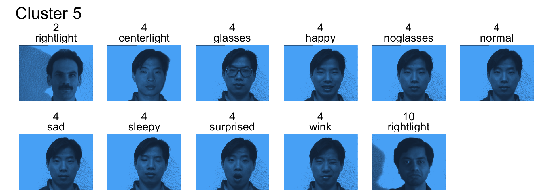
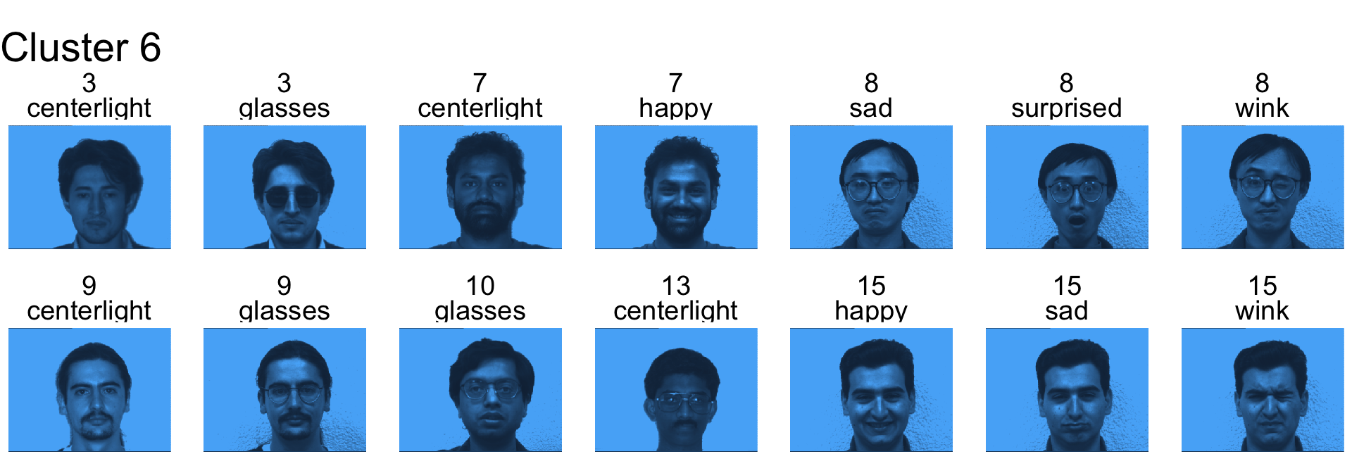
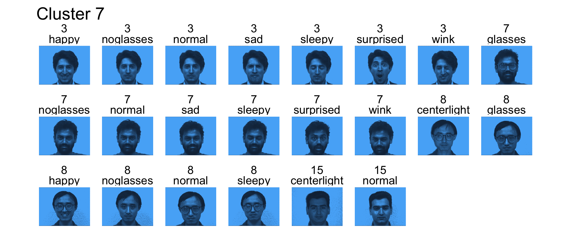
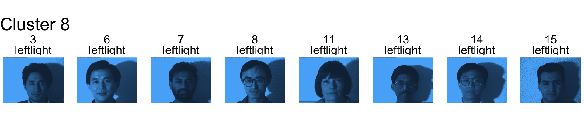
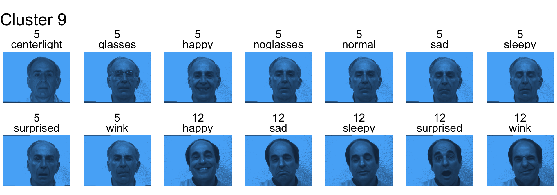
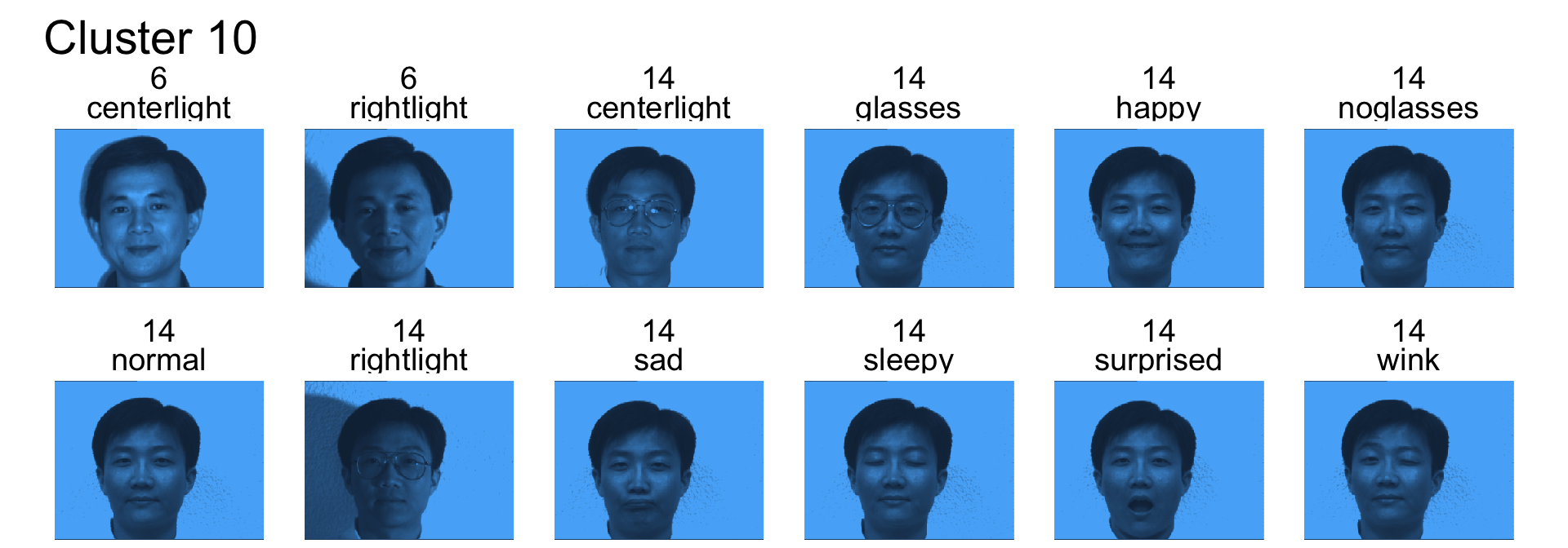
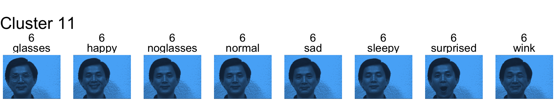
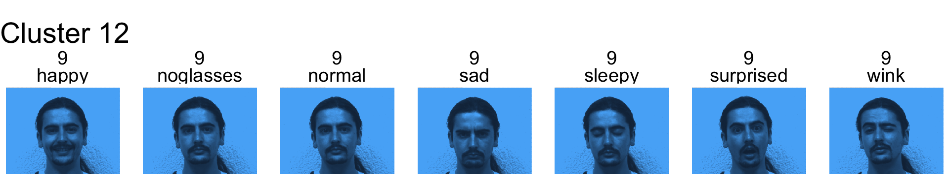
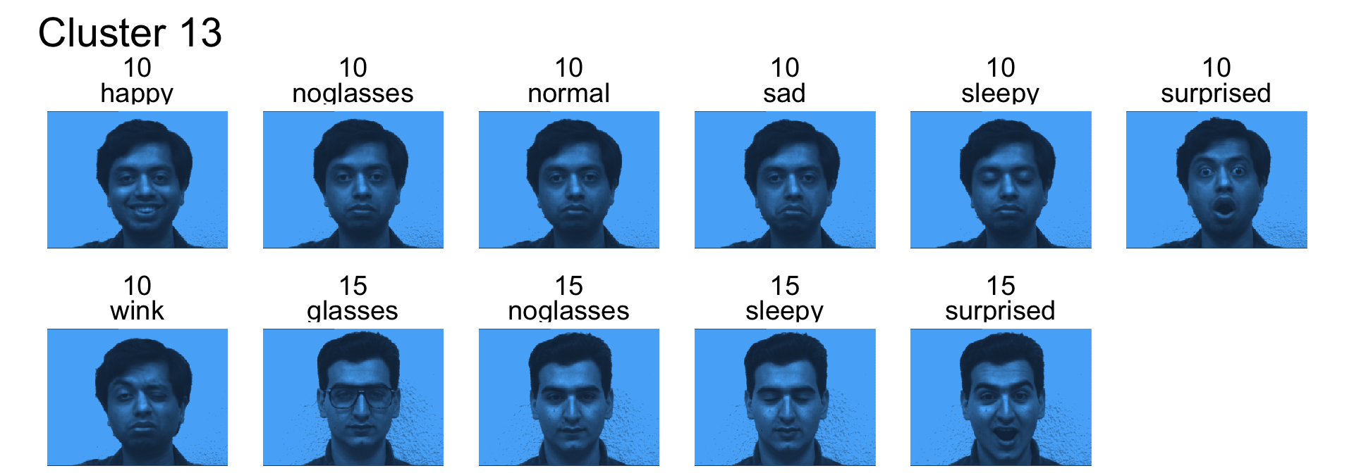
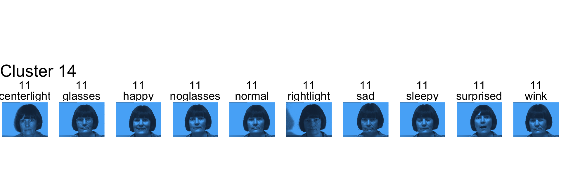
Remember for the following we never used subject id variable in the clustering.
Cluster 1 is mostly subject 1!
- Cluster 2 seems to be capturing mostly the left light.
- Cluster 3 is mostly subject 2.
- Cluster 4 is mostly right light.
- Cluster 5 is mostly subject 4
- Cluster 6 is a mix
- Cluster 7 contains mostly subject 3, 7 and 8
- Cluster 8 is the left light
- Cluster 9 is subjects 5 and 12
- Cluster 10 is mostly subject 14
- Cluster 11 is subject 6
- Cluster 12 is subject 9
- Cluster 13 is subjects 10 and 15
- Cluster 14 is subject 11
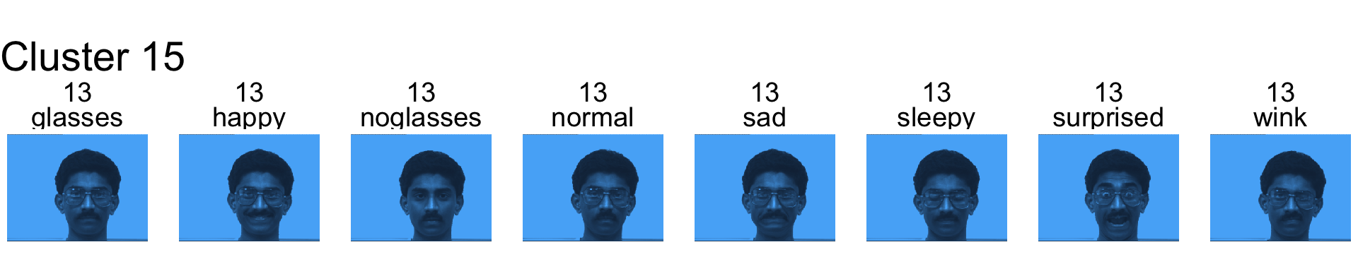
- Cluster 15 is subject 13
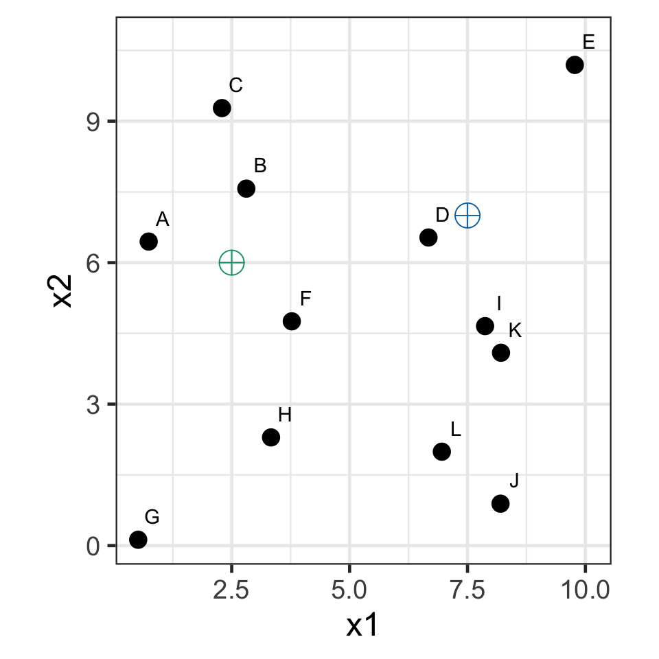
k-means demo: iteration 0
- Select k = 2 with initial seed points (2.5, 6) and (7.5, 7).
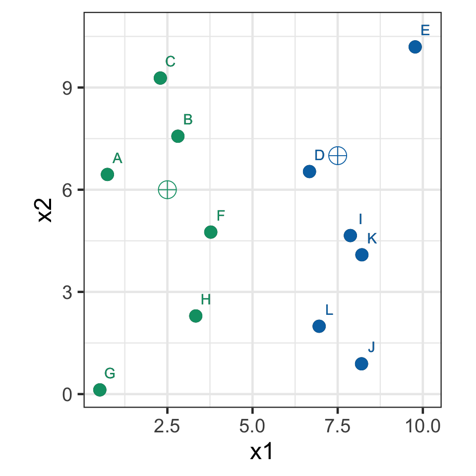
k-means demo: iteration 1
- Assign observations to the closest seed point.
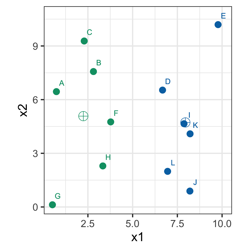
k-means demo: iteration 2
- Recompute the centroids.
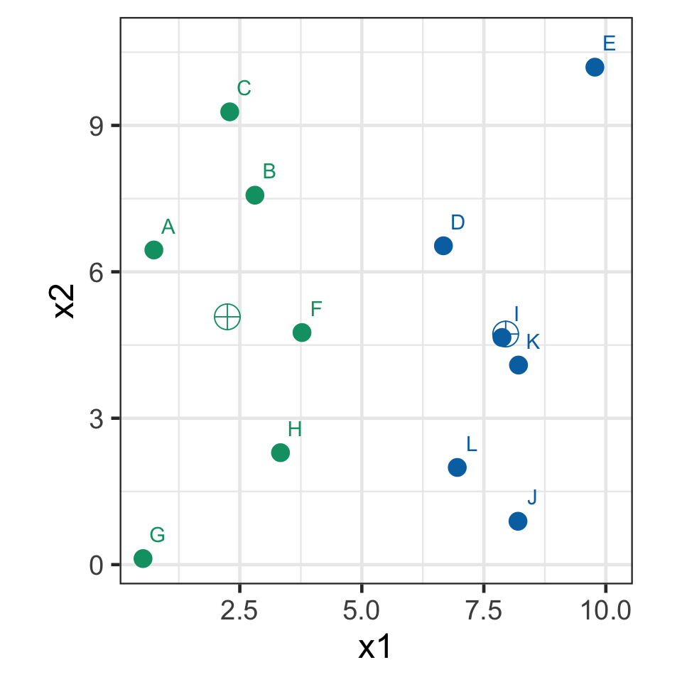
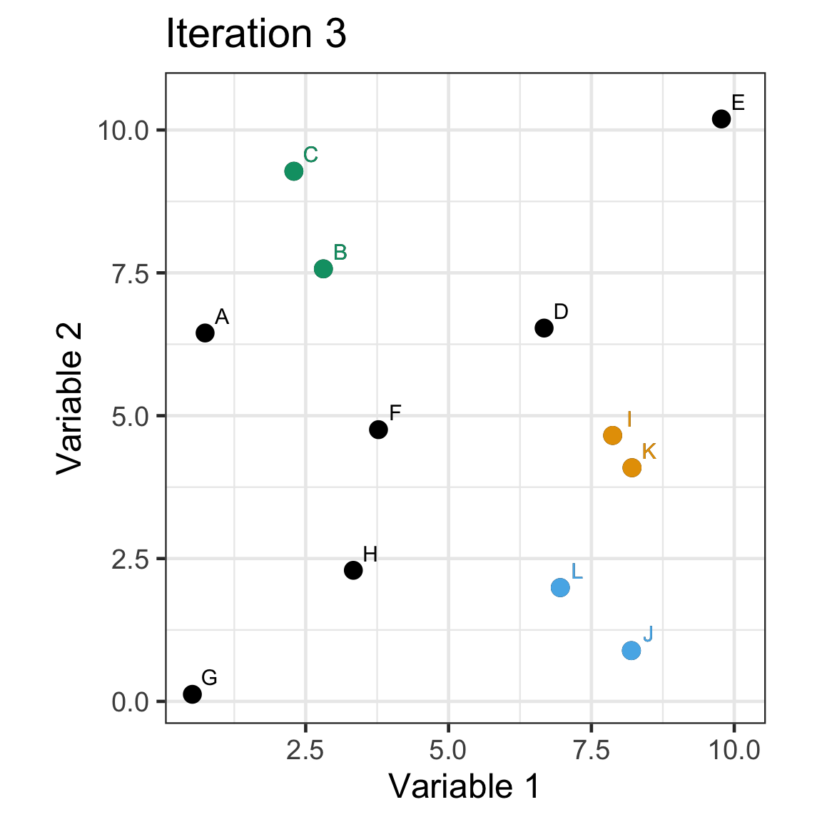
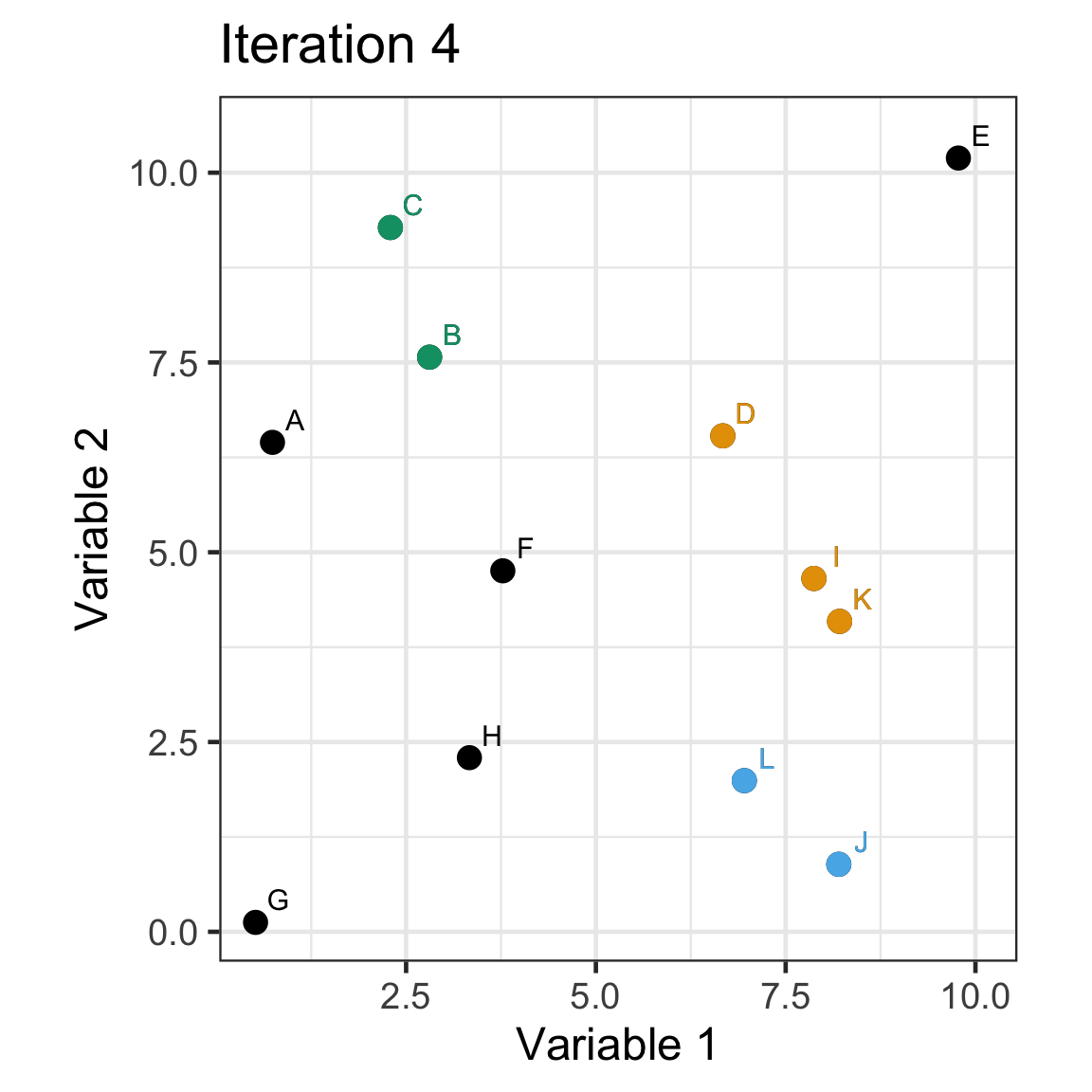
k-means demo: iteration 3
- Assign observations to the closest centroid.
Takeaways
- Clustering is an unsupervised learning.
- There are many methods for clustering.
- Clustering helps to explore data.
- The choice of the number of clusters largely depends on the context of the problem – too many clusters may not be helpful but neither is too few.