| X | Y | Z |
|---|---|---|
| 4 | 8 | 12 |
| 3 | 6 | 9 |
| 5 | 10 | 15 |
| 2 | 4 | 6 |
| 1 | 2 | 3 |
| 6 | 12 | 18 |
ETC3250/5250
Introduction to Machine Learning
Dimension reduction
Lecturer: Emi Tanaka
Department of Econometrics and Business Statistics
High dimensional data
- In marketing, we may conduct a survey with a large number of questions about customer experience.
- In finance, there may be several ways to assess the credit worthiness of firms or individuals.
- In economics, the development of a country or state can be measured by using multiple measures.
Summarising many variables
- Summarising many variables into a single index can be useful.
- For example,
- In finance, a credit score summarises all the information about the likelihood of bankruptcy for a company.
- In economics, the Human Development Index (HDI) is a summary measure that takes nation’s income, education and health into account.
- In actuary, the Australian Actuaries Climate Index summarises the frequency of extreme weather.
Weighted linear combination
- A convenient way to combine variables is through a linear combination of variables.
- For example, your grade for this unit: \text{Final} = w_1\text{Assign 1} + w_2\text{Assign 2} + w_3\text{Assign 2} + w_4\text{Exam}
- Here w_1, w_2, w_3 and w_4 are called weights.
- In this unit, w_1 = w_2 = 0.1, w_3 = 0.2 and w_4 = 0.6.
- What is a good way to choose weights?
- Do we also need to summarise data into a single variable?
Dimension reduction
- Dimension reduction involves mapping the data into a lower dimensional space.
- The mapping, or projection, involves learning the lower dimensional representation of the data.
- This can help in for example,
- efficiency in computation or memory,
- visualisation,
- noise removal, and
- so on.
- efficiency in computation or memory,
Toy example
Alternatively,
\begin{bmatrix}1 & 2 & 3\end{bmatrix} \times
| t1 |
|---|
| 4 |
| 3 |
| 5 |
| 2 |
| 1 |
| 6 |
Geometrically
Original: 3D space
Projection: 1D space
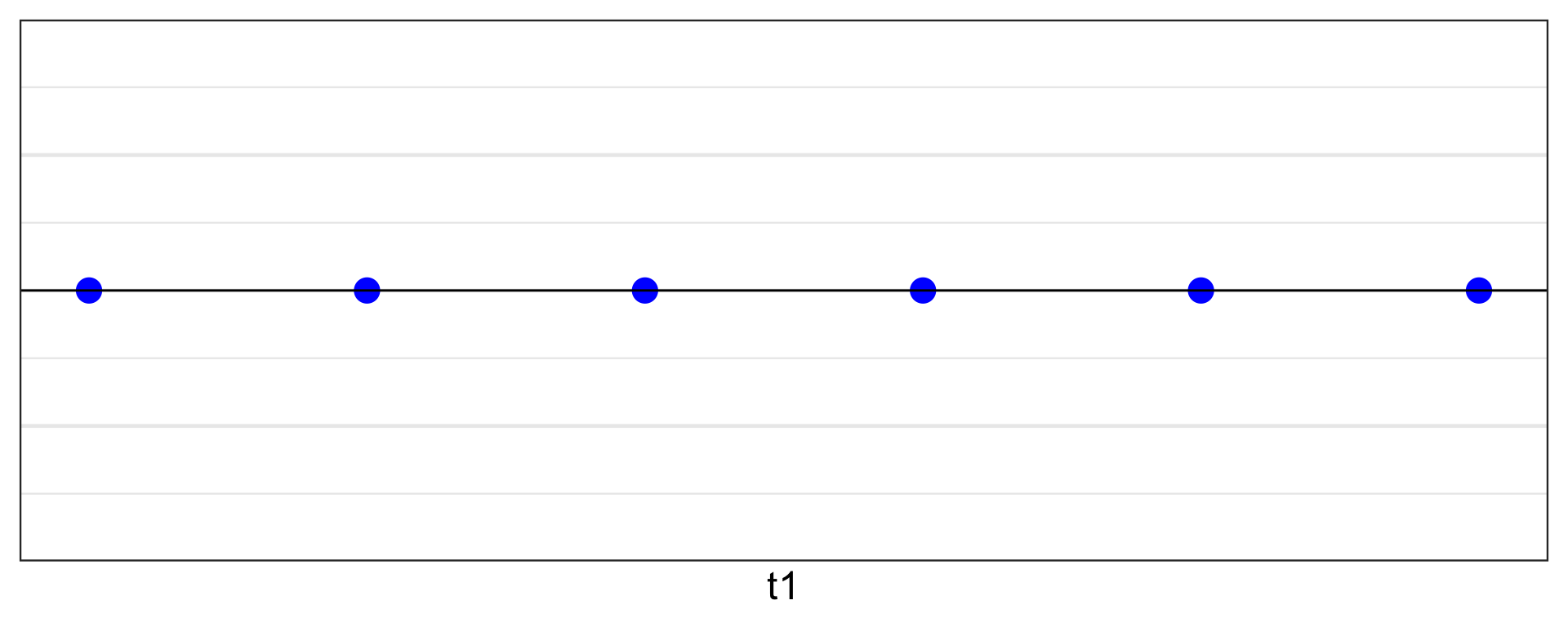
\mathbb{R}^3 \rightarrow \mathbb{R}
But how do we find this projection?
Matrix transformations
A toy data
# A tibble: 600 × 2
      x1    x2
   <dbl> <dbl>
 1    -2 -2
 2    -2 -1.92
 3    -2 -1.84
 4    -2 -1.76
 5    -2 -1.67
 6    -2 -1.59
 7    -2 -1.51
 8    -2 -1.43
 9    -2 -1.35
10    -2 -1.27
# ℹ 590 more rows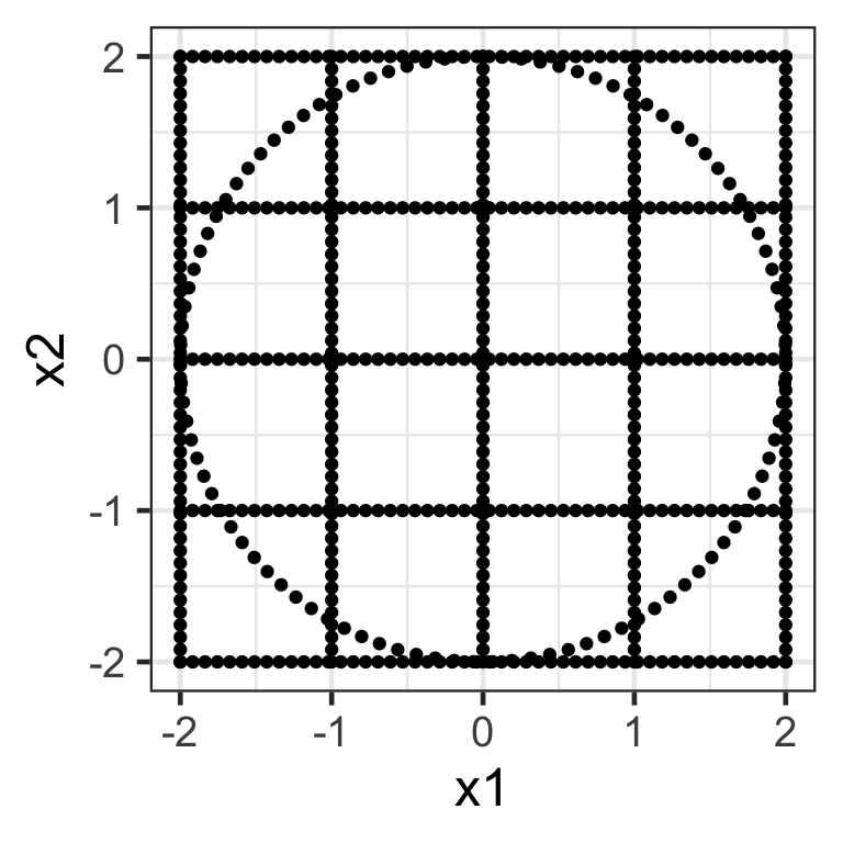
Scaling matrix
- A diagonal matrix where non-diagonal elements are all zero, e.g. \mathbf{S}_{2\times2} = \begin{bmatrix}s_{x_1} & 0 \\ 0 & s_{x_2}\end{bmatrix}.
- Here we apply the transformation \mathbf{X}_{n\times 2}\mathbf{S}_{2\times2} where \mathbf{S}_{2\times2} = \begin{bmatrix}1.5 & 0 \\ 0 & 0.5\end{bmatrix}.
Rotation matrix
- Applying the transformation \mathbf{X}_{n\times 2}\mathbf{R}_{2\times 2} where \mathbf{R}_{2\times2} = \begin{bmatrix}\cos(\theta) & -\sin(\theta) \\\sin(\theta) & \cos(\theta) \end{bmatrix} rotates the data around the origin by an angle of \theta in the counterclockwise direction.
Shear matrix
- A shear matrix can tilt an axis, e.g. \mathbf{H}_{2\times 2} = \begin{bmatrix}1 & \lambda \\ 0 & 1\end{bmatrix} tilts the x-axis.
- The shear matrix below will tilt the y-axis dimension: \mathbf{H}_{2\times 2} = \begin{bmatrix}1 & 0 \\ \lambda & 1\end{bmatrix}.
Inverting transformations
- Suppose we have a new transformed data \hat{\mathbf{X}}_{n\times p} = \mathbf{X}_{n\times p}\mathbf{W}_{p\times p}.
- Then we can get the data in the original measurement by applying: \mathbf{X}_{n\times p} = \hat{\mathbf{X}}_{n\times p}\mathbf{W}^{-1}_{p\times p} provided that \mathbf{W}^{-1} exists.
Matrix decompositions
Eigenvectors and eigenvalues
- For a square matrix, \mathbf{A}, if there exists a vector \boldsymbol{v} and scalar value \lambda such that \mathbf{A}\boldsymbol{v} = \lambda\boldsymbol{v} then \boldsymbol{v} is an eigenvector of \mathbf{A} with eigenvalue of \lambda.
Eigenvalue decomposition
Also called eigendecomposition, diagonalisation or spectral decomposition.
For a positive semi-definite symmetric matrix, \mathbf{V}, there exists an orthogonal matrix \mathbf{Q} and a diagonal matrix \mathbf{\Lambda} such that \mathbf{V} = \mathbf{Q}\mathbf{\Lambda}\mathbf{Q}^{-1}.
\mathbf{\Lambda} is a diagonal matrix where the diagonal entries correspond to eigenvalues.
The columns of \mathbf{Q} are eigenvectors of \mathbf{V} corresponding to the eigenvalues in \mathbf{\Lambda}.
Singular value decomposition
\mathbf{A}_{m\times n} = \mathbf{U}_{m\times m}\mathbf{\Sigma}_{m\times n}\mathbf{V}^\top_{n\times n}
- where
- \mathbf{V} is an orthogonal matrix (i.e. \mathbf{V}^\top\mathbf{V} = \mathbf{I}),
- \mathbf{\Sigma} is a rectangular diagonal matrix, and
- \mathbf{U} is another orthogonal matrix.
- SVD is the same as eigenvalue decomposition if \mathbf{A} is symmetric positive-semidefinite matrix.
Principal components analysis
Principal components
- The k-th principal component is a linear combination of variables: \boldsymbol{t}_k = w_{1k}\boldsymbol{x}_1 + w_{2k}\boldsymbol{x}_2 + \dots + w_{pk}\boldsymbol{x}_p = \mathbf{X}_{n\times p}\boldsymbol{w}_k where \mathbf{X}_{n\times p} = \begin{bmatrix}\boldsymbol{x}_1 & \cdots & \boldsymbol{x}_p \end{bmatrix} and \boldsymbol{w}_k = (w_{1k}, \dots, w_{pk})^\top.
- The elements in \boldsymbol{w}_k are referred to as the loadings (or weights) of the k-th principal component.
- This does assumes all variables are numeric!
Loading or weight matrix
- The matrix \mathbf{W} = \begin{bmatrix}\boldsymbol{w}_1 & \cdots & \boldsymbol{w}_{\min\{n,p\}}\end{bmatrix} is referred to as the loading or weight matrix.
- We obtain the principal component scores (or rotated data) as \mathbf{T} = \begin{bmatrix} \boldsymbol{t}_1 & \cdots & \boldsymbol{t}_{\min\{n,p\}} \end{bmatrix} = \mathbf{X}\mathbf{W}.
First principal components
- The loadings for the first principal component scores are found by maximising the projected variance:
\boldsymbol{w}_1 = \argmax_{\boldsymbol{w}_1} \big\{var(\boldsymbol{t}_1)\big\} = \argmax_{\boldsymbol{w}_1} \big\{var(\mathbf{X}\boldsymbol{w}_1)\big\}.
- Subject to \sum_{j=1}^pw_{j1}^2 = 1.
Second principle component
- The loadings of the second principal component is found from
\boldsymbol{w}_2 = \argmax_{\boldsymbol{w}_2} \big\{var(\boldsymbol{t}_2)\big\} = \argmax_{\boldsymbol{w}_2} \big\{var(\mathbf{X}\boldsymbol{w}_2)\big\}.
- such that \displaystyle\sum_{j=1}^pw_{j2}^2 = 1 and \boldsymbol{w}_1^\top \boldsymbol{w}_2 = 0 (i.e. \boldsymbol{t}_2 is uncorrelated with \boldsymbol{t}_1).
Third principle component and beyond
- The loadings of the third principal component is found from
\boldsymbol{w}_3 = \argmax_{\boldsymbol{w}_3} \big\{var(\boldsymbol{t}_3)\big\} = \argmax_{\boldsymbol{w}_3} \big\{var(\mathbf{X}\boldsymbol{w}_3)\big\}.
- such that \displaystyle\sum_{j=1}^pw_{j3}^2 = 1 and \boldsymbol{t}_3 is uncorrelated with both \boldsymbol{t}_1 and \boldsymbol{t}_2.
- And so on for other higher order PCs.
PCs, eigenvectors and eigenvalues
- Suppose you have a n\times p data matrix \mathbf{X} with each column centered around 0.
- The empirical variance-covariance matrix of the variables is given as \frac{1}{n}\mathbf{X}^\top\mathbf{X}.
- For PCA, we maximise \frac{1}{n}\boldsymbol{w}_k^\top\mathbf{X}^\top\mathbf{X}\boldsymbol{w}_k such that \boldsymbol{w}_k^\top\boldsymbol{w}_k = 1.
- The Lagrangian for this is \frac{1}{n}\boldsymbol{w}_k^\top\mathbf{X}^\top\mathbf{X}\boldsymbol{w}_k-\lambda(\boldsymbol{w}_k^\top\boldsymbol{w}_k - 1).
- The partial derivative with respect to \boldsymbol{w}_k and setting it to zero is 2(\frac{1}{n}\mathbf{X}^\top\mathbf{X} - \lambda\mathbf{I}_n) \boldsymbol{w}_k = 0.
- Therefore, \boldsymbol{w}_k must be an eigenvector of \mathbf{X}^\top\mathbf{X} with eigenvalue of n\lambda.
PCs and SVD
- The PC scores are given as: \mathbf{T} = \mathbf{X}\mathbf{W}.
- Let \mathbf{X} = \mathbf{U}\mathbf{\Sigma}\mathbf{V}^\top.
- It turns out that:
- the columns of \mathbf{U} are the eigenvectors of \mathbf{X}\mathbf{X}^\top,
- the squares of the diagonal elements of \mathbf{\Sigma} are the eigenvalues of both \mathbf{X}^\top\mathbf{X} and \mathbf{X}\mathbf{X}^\top,
- the columns of \mathbf{V} are the eigenvectors of \mathbf{X}^\top\mathbf{X}, and
- \mathbf{W} = \mathbf{V}!
Rotated data
- And so \mathbf{T} = \mathbf{U}\mathbf{\Sigma}\mathbf{W}^\top\mathbf{W} = \mathbf{U}\mathbf{\Sigma}.
- Note that then \mathbf{X} = \mathbf{T}\mathbf{W}^\top.
- You’ll go through more of this in the tutorial.
Geometric interpretation
Alternatively,
- Let \hat{\mathbf{X}}_2 = \mathbf{X} - \mathbf{X}\boldsymbol{w}_1\boldsymbol{w}_1^\top.
- Then \boldsymbol{w}_2 = \argmax_{\boldsymbol{w}_2} \big\{var(\hat{\mathbf{X}}_2\boldsymbol{w}_2)\big\}\text{ such that }\sum_{j=1}^pw_{j2}^2 = 1.
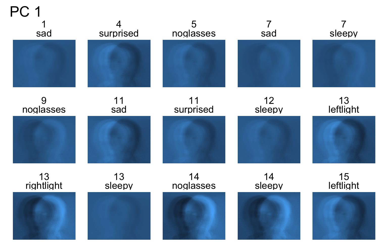
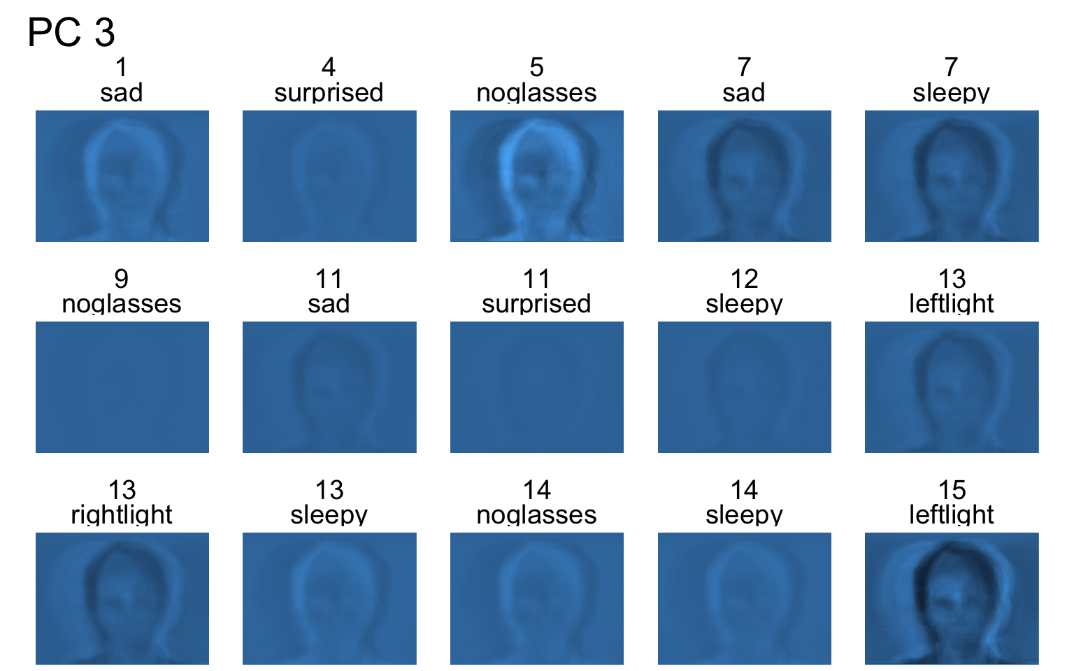
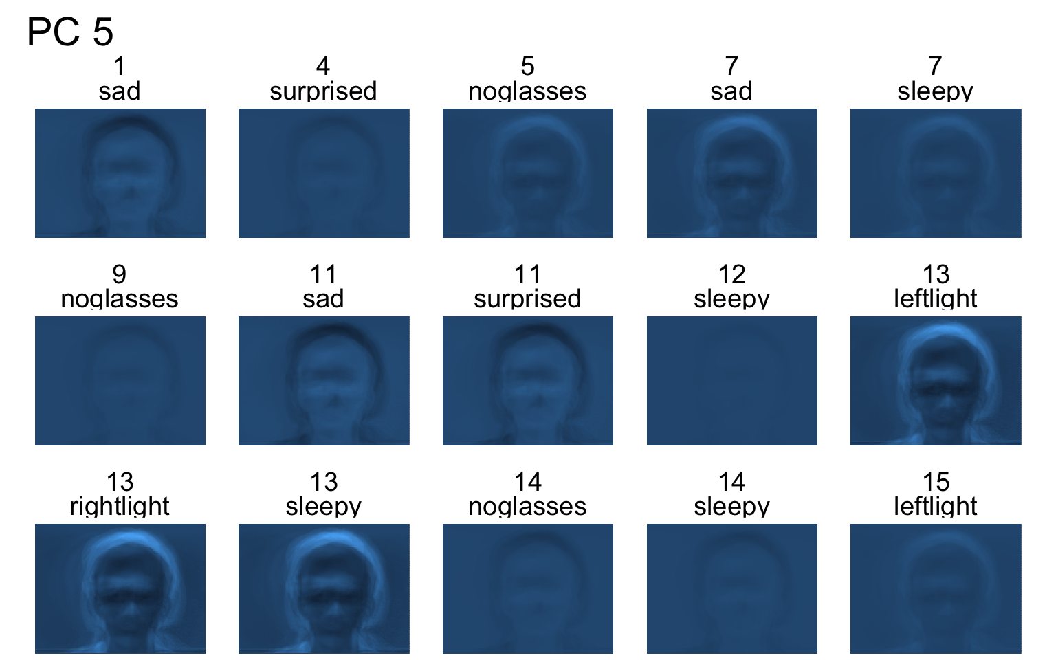
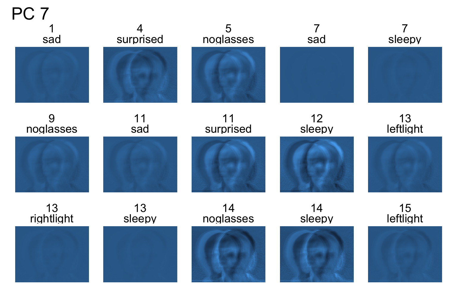
An application to Yale face database
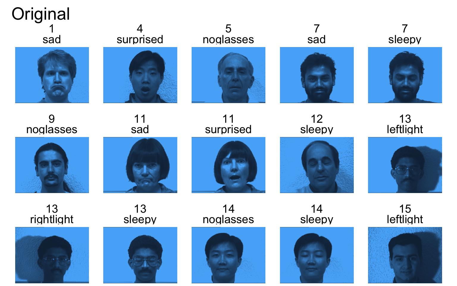
Yale face database
- The data is from P. Belhumeur, J. Hespanha, D. Kriegman, “Eigenfaces vs. Fisherfaces: Recognition Using Class Specific Linear Projection,” IEEE Transactions on Pattern Analysis and Machine Intelligence, July 1997, pp. 711-720.
- The data consists of 15 subjects each under 11 conditions (e.g. “happy”, “sad”, “centerlight”), so a total of 165 images.
- Each image is 320 (width) x 243 (height) = 77,760 pixels (features).
- Note that here n << p!
Sample faces
Code
imagedata_to_plotdata <- function(data = yalefaces,
                                  w = 320,
                                  h = 243,
                                  which = sample(1:165, 15)) {
  data %>%
    mutate(id = 1:n()) %>%
    filter(id %in% which) %>%
    pivot_longer(starts_with("V")) %>%
    mutate(col = rep(rep(1:w, each = h), n_distinct(id)),
           row = rep(rep(1:h, times = w), n_distinct(id)))
}

gfaces <- imagedata_to_plotdata(yalefaces) %>%
    ggplot(aes(col, row)) +
    geom_tile(aes(fill = value)) +
    facet_wrap(~subject + type, nrow = 3) +
    scale_y_reverse() +
    theme_void(base_size = 18) +
    guides(fill = "none") +
    coord_equal()

gfaces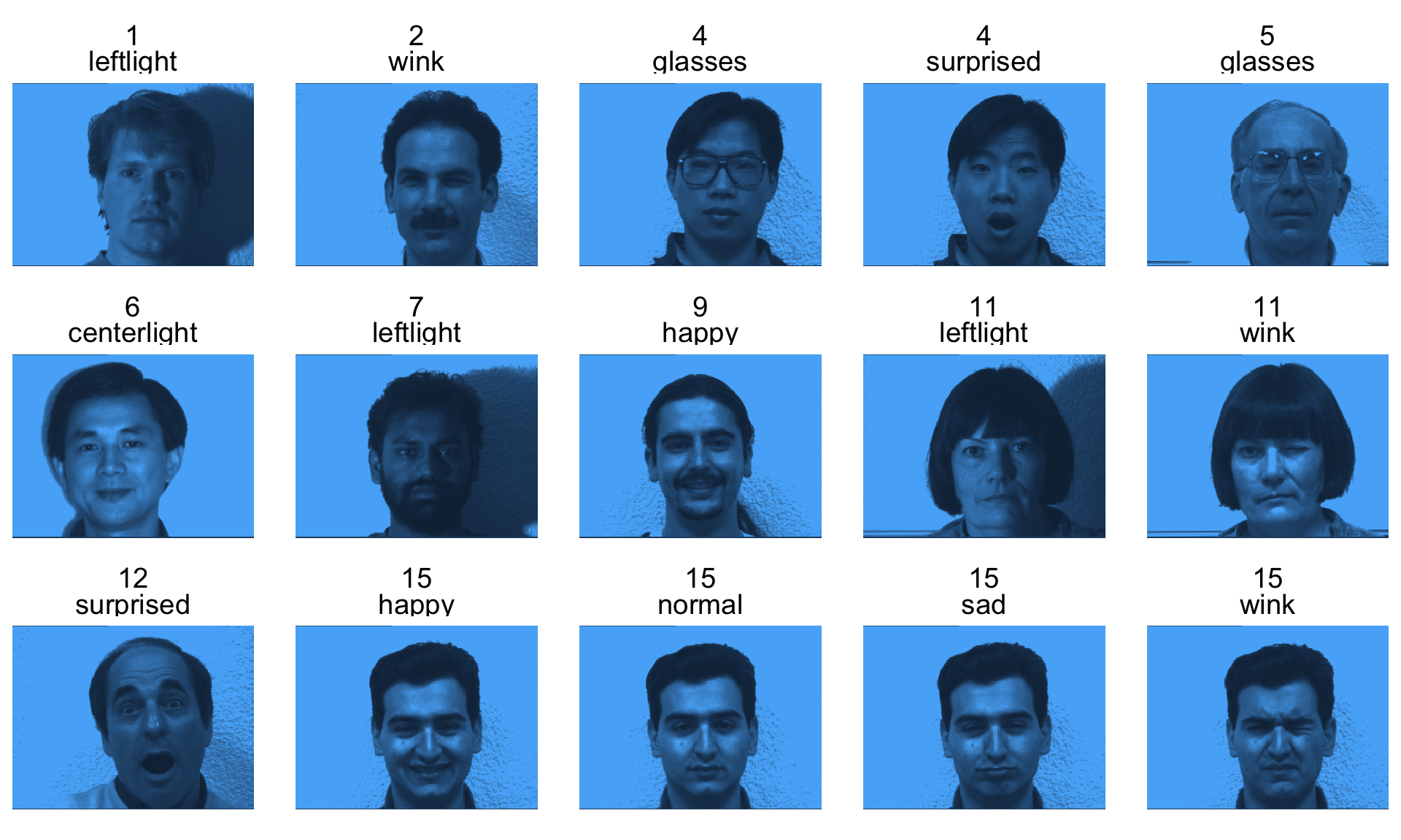
Principle component analysis with R
scroll
- There are several functions for doing principal components analysis in R – we use
prcomp().
yalefaces_x <- yalefaces %>%
  select(-c(subject, type))
yalefaces_pca <- prcomp(yalefaces_x)

str(yalefaces_pca)
List of 5
$ sdev : num [1:165] 10238 6942 5517 5055 4023 ...
$ rotation: num [1:77760, 1:165] -0.000365 -0.000526 -0.000532 -0.000507 -0.00048 ...
..- attr(*, "dimnames")=List of 2
.. ..$ : chr [1:77760] "V1" "V2" "V3" "V4" ...
.. ..$ : chr [1:165] "PC1" "PC2" "PC3" "PC4" ...
$ center : Named num [1:77760] 123 249 250 249 249 ...
..- attr(*, "names")= chr [1:77760] "V1" "V2" "V3" "V4" ...
$ scale : logi FALSE
$ x : num [1:165, 1:165] -7672 -3314 -3065 -16383 -7397 ...
..- attr(*, "dimnames")=List of 2
.. ..$ : NULL
.. ..$ : chr [1:165] "PC1" "PC2" "PC3" "PC4" ...
- attr(*, "class")= chr "prcomp"prcompobject contains:sdevare the standard deviations of the principle componentsrotationis the loading matrixxis the rotated data (centered + scaled data multiplied byrotationmatrix)centeris the centering (if any)scaleis a logical value to indicate if scaling was done
Summary of PCA
- The summary of
prcompobject shows for each PC,- it’s standard deviation,
- the proportion of variation it explains, and
- the cumulative proportion of variation it explains.
- Below shows that PCs of up to (and including) 50 explains 95.11% of the variation in the data.
Importance of components:
                             PC1       PC2       PC3       PC4       PC5
Standard deviation     1.024e+04 6942.0245 5.517e+03 5.055e+03 4.023e+03
Proportion of Variance 3.054e-01    0.1404 8.869e-02 7.444e-02 4.715e-02
Cumulative Proportion  3.054e-01    0.4458 5.345e-01 6.089e-01 6.561e-01
                             PC6       PC7       PC8       PC9      PC10
Standard deviation     3.762e+03 3.081e+03 2.812e+03 2.771e+03 2.523e+03
Proportion of Variance 4.123e-02 2.766e-02 2.304e-02 2.237e-02 1.855e-02
Cumulative Proportion  6.973e-01 7.250e-01 7.480e-01 7.704e-01 7.889e-01
                            PC11      PC12      PC13      PC14      PC15
Standard deviation     2.150e+03 1.998e+03 1.795e+03 1.760e+03 1.731e+03
Proportion of Variance 1.346e-02 1.163e-02 9.390e-03 9.030e-03 8.730e-03
Cumulative Proportion  8.024e-01 8.140e-01 8.234e-01 8.325e-01 8.412e-01
                            PC16      PC17      PC18      PC19      PC20
Standard deviation     1657.4044 1.586e+03 1.502e+03 1.463e+03 1.432e+03
Proportion of Variance    0.0080 7.320e-03 6.570e-03 6.240e-03 5.970e-03
Cumulative Proportion     0.8492 8.565e-01 8.631e-01 8.693e-01 8.753e-01
                            PC21      PC22      PC23      PC24      PC25
Standard deviation     1.343e+03 1.291e+03 1.235e+03 1.205e+03 1.147e+03
Proportion of Variance 5.260e-03 4.850e-03 4.450e-03 4.230e-03 3.840e-03
Cumulative Proportion  8.806e-01 8.854e-01 8.899e-01 8.941e-01 8.979e-01
                            PC26      PC27      PC28      PC29     PC30
Standard deviation     1.144e+03 1.084e+03 1.036e+03 1.018e+03 979.5103
Proportion of Variance 3.810e-03 3.420e-03 3.130e-03 3.020e-03   0.0028
Cumulative Proportion  9.017e-01 9.052e-01 9.083e-01 9.113e-01   0.9141
                            PC31      PC32     PC33      PC34      PC35
Standard deviation     973.46557 949.70604 926.0579 899.08034 886.35745
Proportion of Variance   0.00276   0.00263   0.0025   0.00236   0.00229
Cumulative Proportion    0.91685   0.91948   0.9220   0.92433   0.92662
                            PC36      PC37      PC38      PC39      PC40
Standard deviation     854.35433 819.97982 804.40097 797.11137 781.00509
Proportion of Variance   0.00213   0.00196   0.00189   0.00185   0.00178
Cumulative Proportion    0.92874   0.93070   0.93259   0.93444   0.93622
                            PC41      PC42     PC43      PC44     PC45
Standard deviation     767.79261 753.83380 741.3496 728.30022 717.7012
Proportion of Variance   0.00172   0.00166   0.0016   0.00155   0.0015
Cumulative Proportion    0.93794   0.93959   0.9412   0.94274   0.9442
                            PC46      PC47      PC48      PC49      PC50
Standard deviation     708.79276 695.40095 681.32271 679.49515 666.06781
Proportion of Variance   0.00146   0.00141   0.00135   0.00135   0.00129
Cumulative Proportion    0.94570   0.94711   0.94846   0.94981   0.95110
                            PC51      PC52     PC53      PC54      PC55
Standard deviation     659.25153 650.97034 642.5660 634.40640 624.82484
Proportion of Variance   0.00127   0.00123   0.0012   0.00117   0.00114
Cumulative Proportion    0.95237   0.95360   0.9548   0.95598   0.95712
                            PC56      PC57      PC58      PC59      PC60
Standard deviation     604.43618 602.54879 595.95461 589.03690 584.19071
Proportion of Variance   0.00106   0.00106   0.00103   0.00101   0.00099
Cumulative Proportion    0.95818   0.95924   0.96027   0.96128   0.96228
                            PC61      PC62      PC63      PC64      PC65
Standard deviation     583.05237 565.14296 558.41544 550.93341 546.82381
Proportion of Variance   0.00099   0.00093   0.00091   0.00088   0.00087
Cumulative Proportion    0.96327   0.96420   0.96511   0.96599   0.96686
                            PC66      PC67      PC68     PC69      PC70
Standard deviation     538.43362 532.84440 526.71190 524.7713 515.42757
Proportion of Variance   0.00084   0.00083   0.00081   0.0008   0.00077
Cumulative Proportion    0.96771   0.96854   0.96934   0.9701   0.97092
                            PC71      PC72      PC73      PC74     PC75
Standard deviation     510.56175 508.12438 494.47828 491.91604 489.4362
Proportion of Variance   0.00076   0.00075   0.00071   0.00071   0.0007
Cumulative Proportion    0.97168   0.97243   0.97314   0.97385   0.9746
                            PC76      PC77      PC78      PC79      PC80
Standard deviation     481.77831 474.38456 470.41992 466.23367 456.39436
Proportion of Variance   0.00068   0.00066   0.00064   0.00063   0.00061
Cumulative Proportion    0.97522   0.97588   0.97652   0.97716   0.97776
                           PC81     PC82      PC83      PC84      PC85
Standard deviation     454.5586 453.5185 444.90730 441.53940 435.61013
Proportion of Variance   0.0006   0.0006   0.00058   0.00057   0.00055
Cumulative Proportion    0.9784   0.9790   0.97954   0.98011   0.98066
                            PC86      PC87      PC88     PC89      PC90
Standard deviation     429.57105 426.69337 423.89192 413.2288 411.06527
Proportion of Variance   0.00054   0.00053   0.00052   0.0005   0.00049
Cumulative Proportion    0.98120   0.98173   0.98226   0.9828   0.98324
                            PC91      PC92      PC93      PC94      PC95
Standard deviation     408.23987 403.71341 400.32073 397.67775 394.87635
Proportion of Variance   0.00049   0.00047   0.00047   0.00046   0.00045
Cumulative Proportion    0.98373   0.98421   0.98467   0.98513   0.98559
                            PC96      PC97      PC98      PC99     PC100
Standard deviation     390.69468 389.12213 383.96911 382.15048 376.12550
Proportion of Variance   0.00044   0.00044   0.00043   0.00043   0.00041
Cumulative Proportion    0.98603   0.98647   0.98690   0.98733   0.98774
                          PC101     PC102     PC103     PC104     PC105
Standard deviation     371.2632 365.76624 363.96111 360.61787 355.51007
Proportion of Variance   0.0004   0.00039   0.00039   0.00038   0.00037
Cumulative Proportion    0.9881   0.98853   0.98892   0.98930   0.98967
                           PC106     PC107     PC108     PC109     PC110
Standard deviation     349.66834 347.69259 344.76632 342.22007 336.67809
Proportion of Variance   0.00036   0.00035   0.00035   0.00034   0.00033
Cumulative Proportion    0.99002   0.99037   0.99072   0.99106   0.99139
                           PC111     PC112     PC113     PC114    PC115
Standard deviation     333.36005 331.10318 330.25164 326.73677 322.4559
Proportion of Variance   0.00032   0.00032   0.00032   0.00031   0.0003
Cumulative Proportion    0.99172   0.99203   0.99235   0.99266   0.9930
                          PC116     PC117     PC118     PC119     PC120
Standard deviation     319.0804 317.32550 310.97104 310.16044 306.05539
Proportion of Variance   0.0003   0.00029   0.00028   0.00028   0.00027
Cumulative Proportion    0.9933   0.99356   0.99384   0.99412   0.99439
                           PC121     PC122     PC123     PC124     PC125
Standard deviation     303.24091 299.56704 297.28634 293.09425 286.00109
Proportion of Variance   0.00027   0.00026   0.00026   0.00025   0.00024
Cumulative Proportion    0.99466   0.99492   0.99518   0.99543   0.99567
                           PC126     PC127     PC128     PC129     PC130
Standard deviation     282.01505 280.37829 275.73911 271.80841 268.07858
Proportion of Variance   0.00023   0.00023   0.00022   0.00022   0.00021
Cumulative Proportion    0.99590   0.99613   0.99635   0.99656   0.99677
                          PC131    PC132    PC133     PC134     PC135     PC136
Standard deviation     265.1800 264.0004 259.6532 255.95912 253.99049 250.14523
Proportion of Variance   0.0002   0.0002   0.0002   0.00019   0.00019   0.00018
Cumulative Proportion    0.9970   0.9972   0.9974   0.99757   0.99776   0.99794
                           PC137     PC138     PC139     PC140     PC141
Standard deviation     243.24003 240.62311 236.08174 232.01663 226.44527
Proportion of Variance   0.00017   0.00017   0.00016   0.00016   0.00015
Cumulative Proportion    0.99811   0.99828   0.99844   0.99860   0.99875
                           PC142    PC143     PC144     PC145     PC146
Standard deviation     222.92802 2.16e+02 201.99100 199.59454 193.46553
Proportion of Variance   0.00014 1.40e-04   0.00012   0.00012   0.00011
Cumulative Proportion    0.99889 9.99e-01   0.99915   0.99926   0.99937
                          PC147    PC148     PC149     PC150     PC151
Standard deviation     186.8505 182.9617 179.78968 177.88182 168.71830
Proportion of Variance   0.0001   0.0001   0.00009   0.00009   0.00008
Cumulative Proportion    0.9995   0.9996   0.99967   0.99976   0.99984
                           PC152     PC153    PC154    PC155     PC156
Standard deviation     139.05249 133.45290 95.80808 87.90070 2.527e-11
Proportion of Variance   0.00006   0.00005  0.00003  0.00002 0.000e+00
Cumulative Proportion    0.99990   0.99995  0.99998  1.00000 1.000e+00
                           PC157     PC158     PC159     PC160     PC161
Standard deviation     8.795e-12 6.398e-12 5.481e-12 2.854e-12 1.897e-12
Proportion of Variance 0.000e+00 0.000e+00 0.000e+00 0.000e+00 0.000e+00
Cumulative Proportion  1.000e+00 1.000e+00 1.000e+00 1.000e+00 1.000e+00
                           PC162     PC163     PC164     PC165
Standard deviation     1.095e-12 9.856e-13 7.621e-13 7.621e-13
Proportion of Variance 0.000e+00 0.000e+00 0.000e+00 0.000e+00
Cumulative Proportion  1.000e+00 1.000e+00 1.000e+00 1.000e+00
Summary of PCA “by hand”
sdevis simply the sample standard deviation of the rotated data:
      PC1       PC2       PC3       PC4       PC5       PC6
10237.892 6942.025 5517.123 5054.695 4022.602 3761.812 [1] 10237.892 6942.025 5517.123 5054.695 4022.602 3761.812- Proportion of variation explained “by hand”:
The total variation of PCs
- There are a total of \min\{p, n\} PCs.
- The total variation of the PCs explain all of the variation of the original variables.
\sum_{j = 1}^{\min\{p,~n\}}var(\boldsymbol{t}_j) = \sum_{j=1}^pvar(\boldsymbol{x}_j)
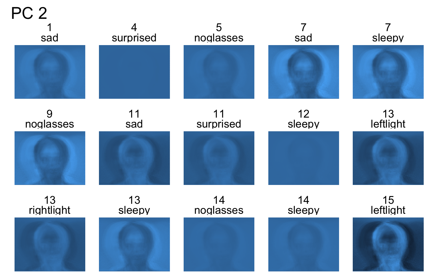
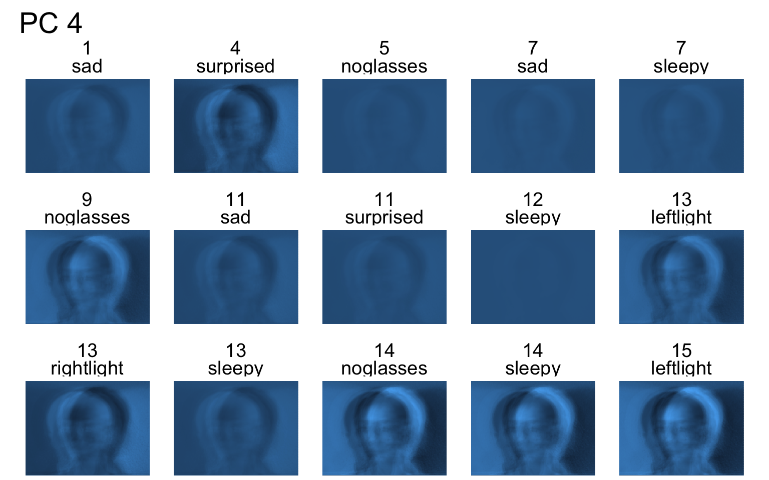
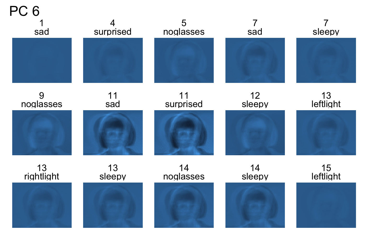
Image compression
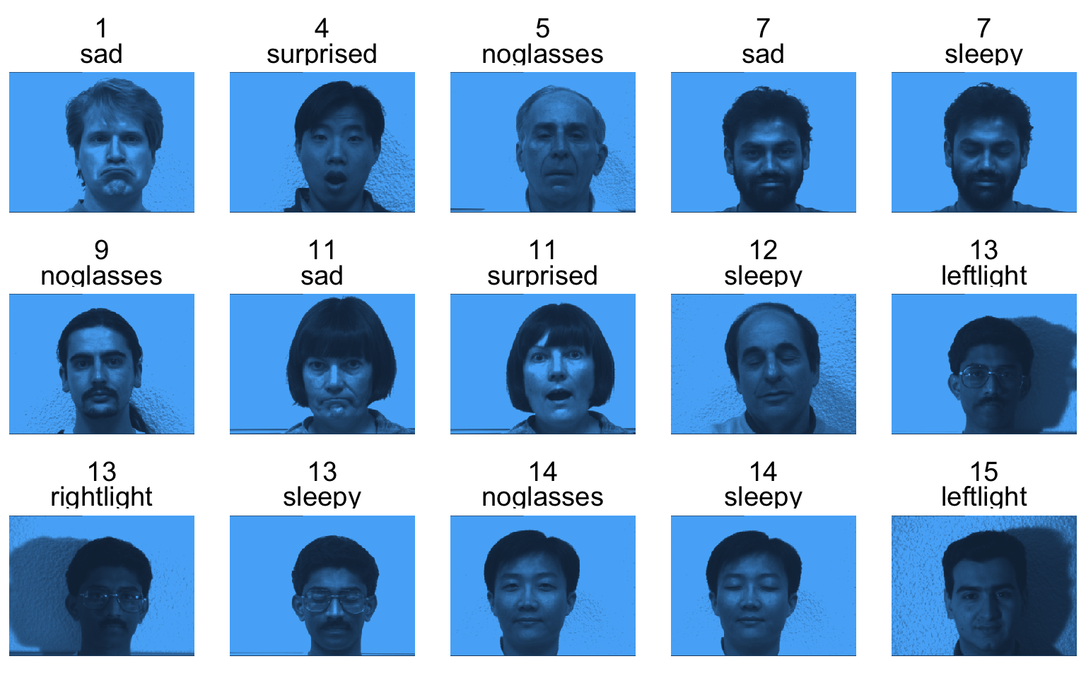
Based on the original data:
165 \times 320 \times 243 \approx 12.8\text{ million}
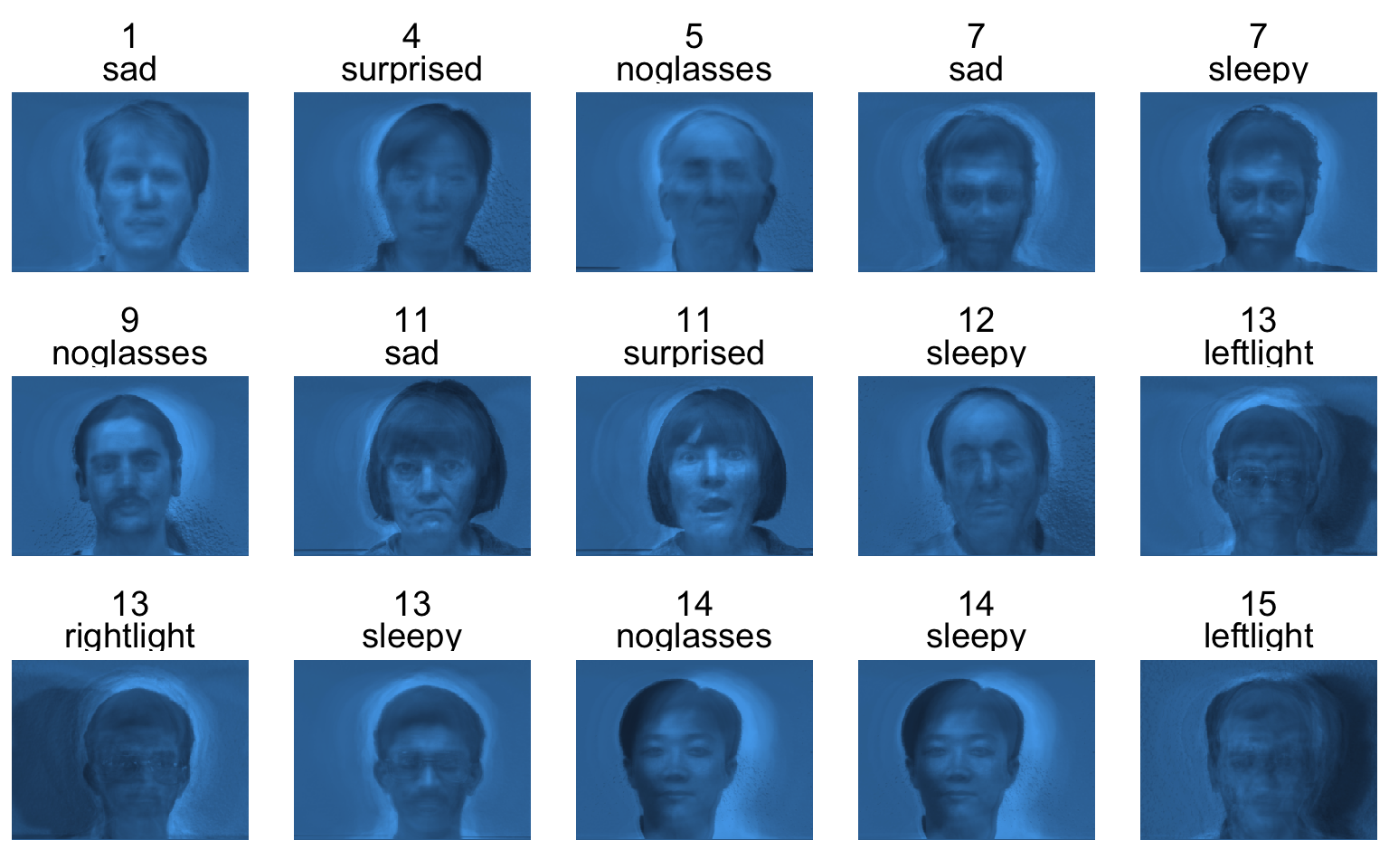
Based on 50 PCs:
165 \times 50 + 50 \times 320 \times 243 \approx 3.9\text{ million}
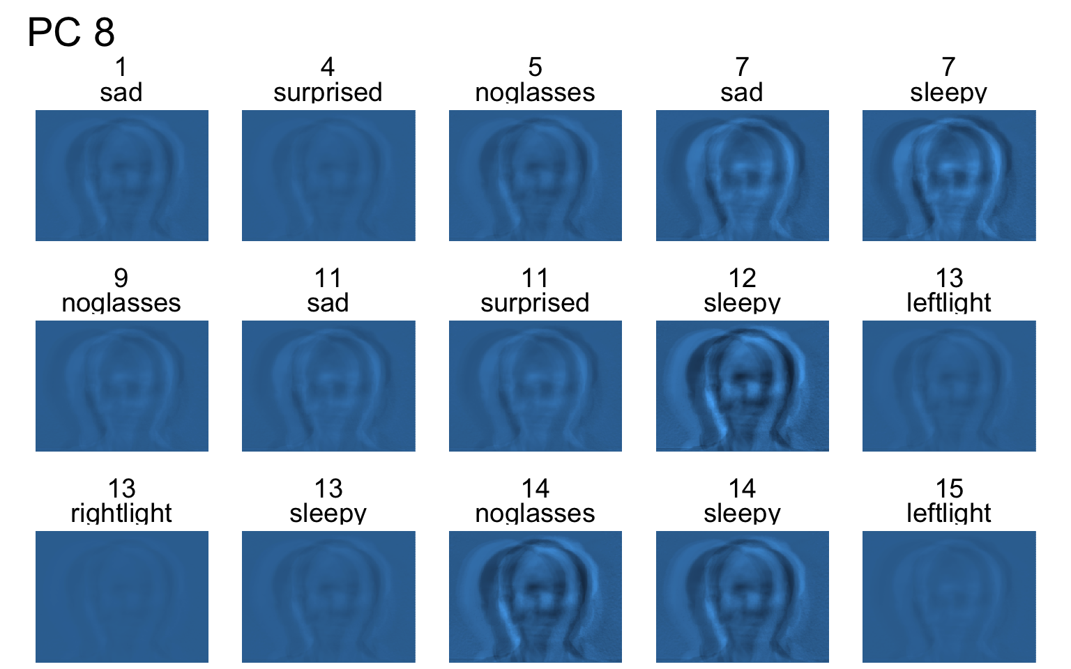
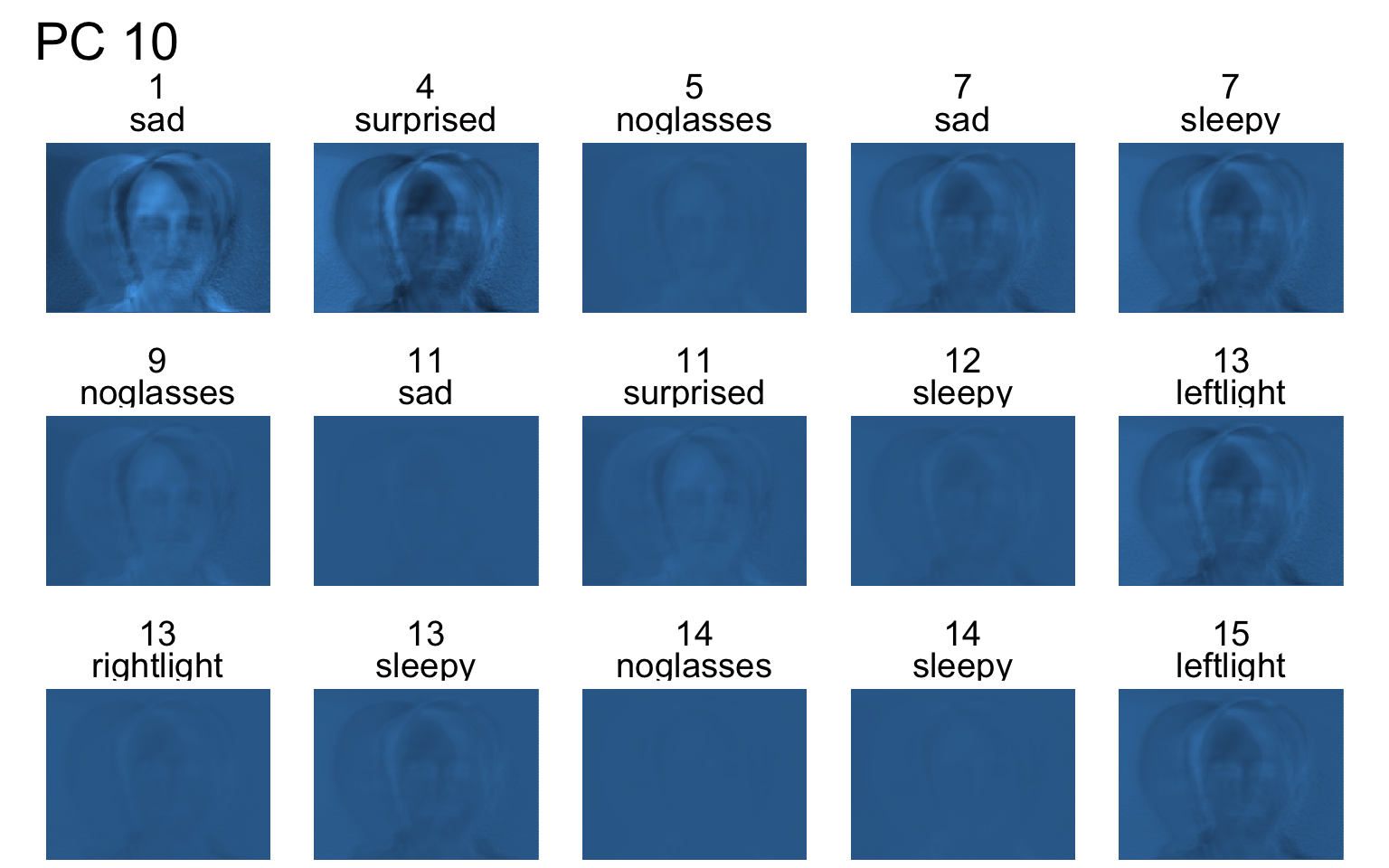
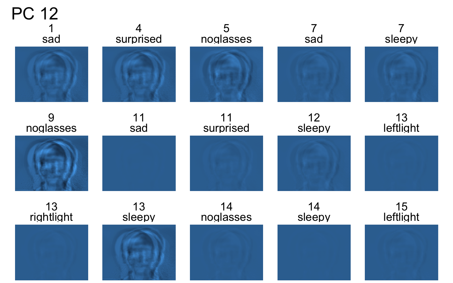
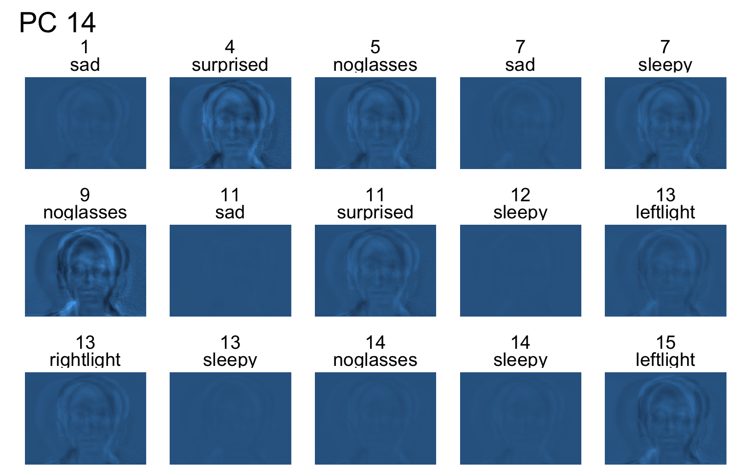
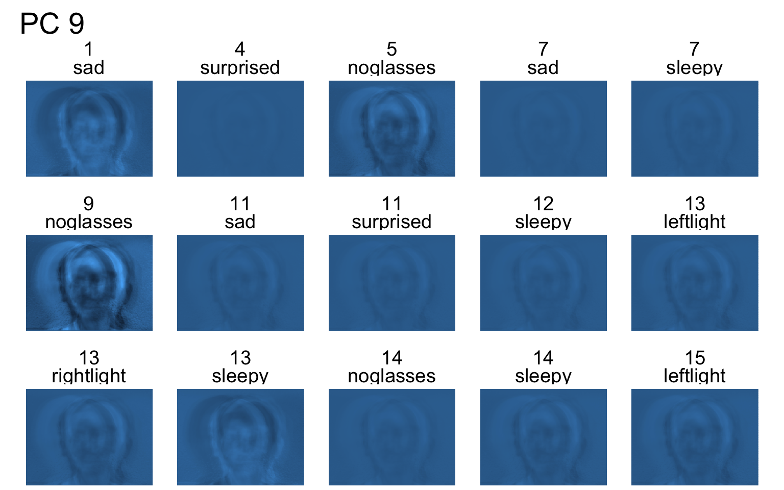
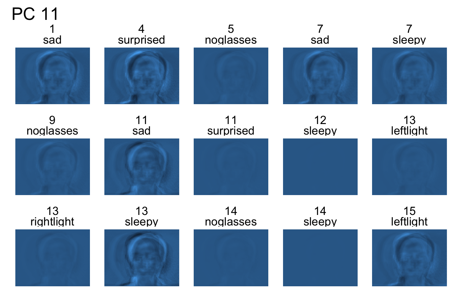
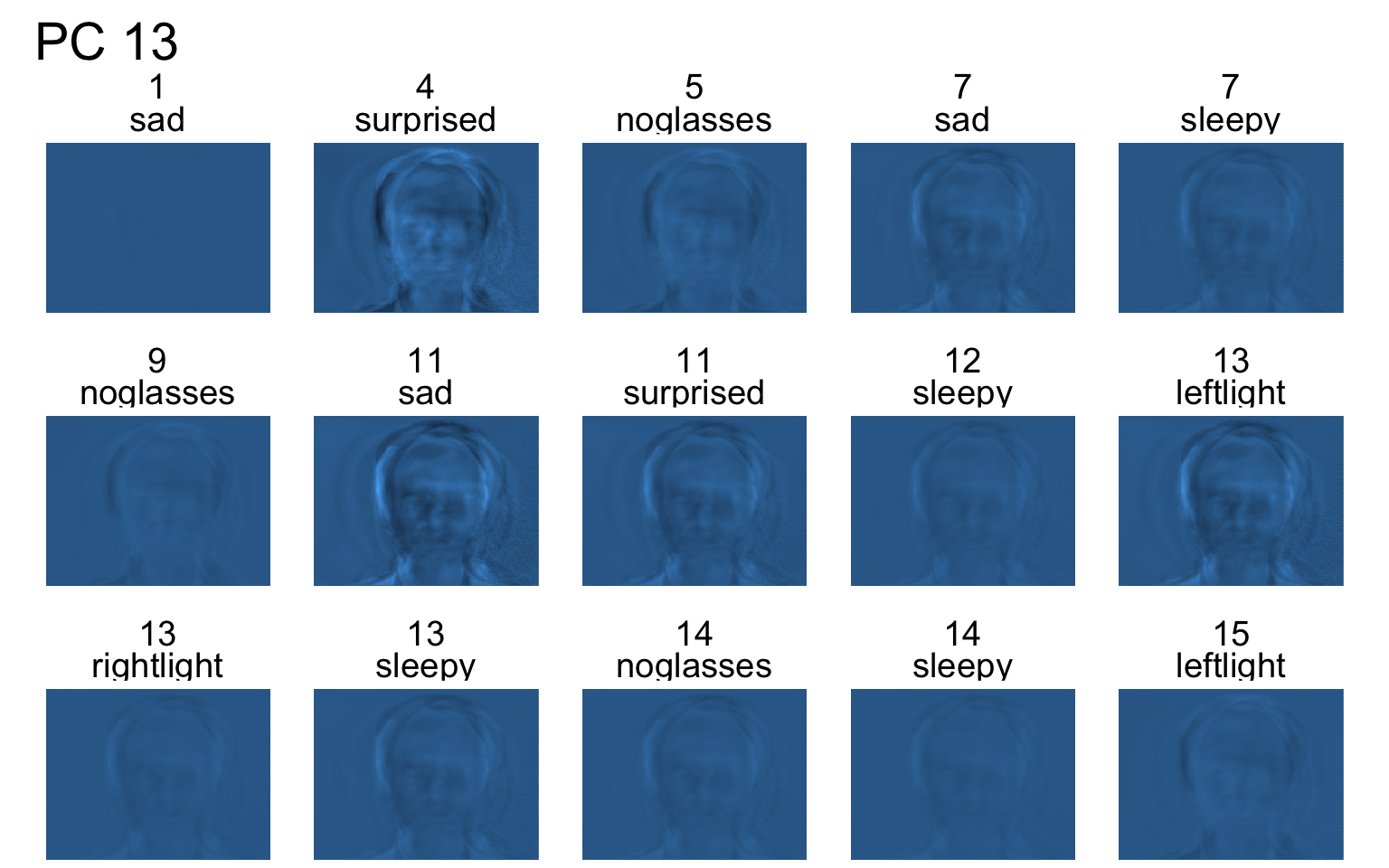
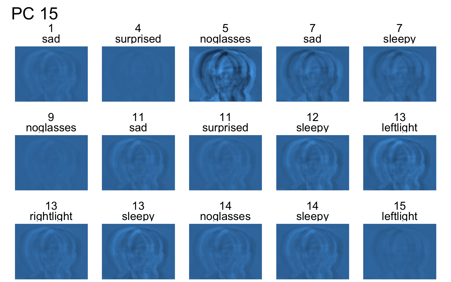
Facial recognition
scroll
- Each PC captures a different aspect of the data.
- The PCs can be treated as a feature downstream, say, for facial recognition systems.
An application to wine quality data
Wine quality data
scroll
This data on wine quality found here.
| Name | wine |
| Number of rows | 6497 |
| Number of columns | 13 |
| _______________________ | |
| Column type frequency: | |
| character | 1 |
| numeric | 12 |
| ________________________ | |
| Group variables | None |
Variable type: character
| skim_variable | n_missing | complete_rate | min | max | empty | n_unique | whitespace |
|---|---|---|---|---|---|---|---|
| type | 0 | 1 | 3 | 5 | 0 | 2 | 0 |
Variable type: numeric
| skim_variable | n_missing | complete_rate | mean | sd | p0 | p25 | p50 | p75 | p100 | hist |
|---|---|---|---|---|---|---|---|---|---|---|
| fixed acidity | 10 | 1 | 7.22 | 1.30 | 3.80 | 6.40 | 7.00 | 7.70 | 15.90 | ▂▇▁▁▁ |
| volatile acidity | 8 | 1 | 0.34 | 0.16 | 0.08 | 0.23 | 0.29 | 0.40 | 1.58 | ▇▂▁▁▁ |
| citric acid | 3 | 1 | 0.32 | 0.15 | 0.00 | 0.25 | 0.31 | 0.39 | 1.66 | ▇▅▁▁▁ |
| residual sugar | 2 | 1 | 5.44 | 4.76 | 0.60 | 1.80 | 3.00 | 8.10 | 65.80 | ▇▁▁▁▁ |
| chlorides | 2 | 1 | 0.06 | 0.04 | 0.01 | 0.04 | 0.05 | 0.06 | 0.61 | ▇▁▁▁▁ |
| free sulfur dioxide | 0 | 1 | 30.53 | 17.75 | 1.00 | 17.00 | 29.00 | 41.00 | 289.00 | ▇▁▁▁▁ |
| total sulfur dioxide | 0 | 1 | 115.74 | 56.52 | 6.00 | 77.00 | 118.00 | 156.00 | 440.00 | ▅▇▂▁▁ |
| density | 0 | 1 | 0.99 | 0.00 | 0.99 | 0.99 | 0.99 | 1.00 | 1.04 | ▇▂▁▁▁ |
| pH | 9 | 1 | 3.22 | 0.16 | 2.72 | 3.11 | 3.21 | 3.32 | 4.01 | ▁▇▆▁▁ |
| sulphates | 4 | 1 | 0.53 | 0.15 | 0.22 | 0.43 | 0.51 | 0.60 | 2.00 | ▇▃▁▁▁ |
| alcohol | 0 | 1 | 10.49 | 1.19 | 8.00 | 9.50 | 10.30 | 11.30 | 14.90 | ▃▇▅▂▁ |
| quality | 0 | 1 | 5.82 | 0.87 | 3.00 | 5.00 | 6.00 | 6.00 | 9.00 | ▁▆▇▃▁ |
- There are small amount missing values in the data.
- For ease of computation, let’s ignore any observations with missing values ( don’t do this in practice!)
Scaling then PCA
wine_pca <- winec %>%
  select(-type) %>%
  scale() %>%
  prcomp() # or skip above line and use prcomp(.scale = TRUE)

wine_pca
Standard deviations (1, .., p=12):
[1] 1.7445303 1.6276285 1.2809541 1.0337025 0.9172812 0.8133844 0.7505644
[8] 0.7178551 0.6768948 0.5460465 0.4767787 0.1808925
Rotation (n x k) = (12 x 12):
PC1 PC2 PC3 PC4
fixed acidity 0.26071445 -0.2589454 0.46564247 -0.14566848
volatile acidity 0.39565721 -0.1017451 -0.28077847 -0.07972791
citric acid -0.14371362 -0.1458295 0.58854048 0.05320974
residual sugar -0.31632548 -0.3455107 -0.07365003 0.11416835
chlorides 0.31574995 -0.2668505 0.04612386 0.16409739
free sulfur dioxide -0.42198110 -0.1158082 -0.09751916 0.30117025
total sulfur dioxide -0.47318123 -0.1486730 -0.10010043 0.13109780
density 0.09751989 -0.5540261 -0.05065537 0.15110768
pH 0.20549880 0.1541321 -0.40589466 0.47551131
sulphates 0.30062120 -0.1172996 0.17132282 0.58618450
alcohol 0.05400002 0.4937868 0.21317892 0.08009431
quality -0.08984644 0.2948571 0.29793560 0.47198353
PC5 PC6 PC7 PC8
fixed acidity 0.164412120 -0.03309162 0.39667040 -0.001027375
volatile acidity 0.147587298 0.37665137 0.44898061 0.308979027
citric acid -0.237540038 -0.36465719 0.04508088 0.442396627
residual sugar 0.507179210 0.06151257 -0.09591307 0.085514113
chlorides -0.391063164 0.42844719 -0.47017478 0.381450232
free sulfur dioxide -0.249063830 0.28146210 0.36627137 0.117939741
total sulfur dioxide -0.224891074 0.10673778 0.23527950 0.011180004
density 0.329530808 -0.15600804 0.01445317 0.041722486
pH -0.005058406 -0.56226140 0.07866747 0.357336224
sulphates -0.195771884 0.02503005 0.16520174 -0.592620308
alcohol 0.113678532 0.16527545 0.33900469 0.229085262
quality 0.460571232 0.27871185 -0.26579816 0.094104102
PC9 PC10 PC11 PC12
fixed acidity -0.4227271729 -0.27139305 -0.276874322 0.3353301943
volatile acidity 0.1286615123 0.49373092 0.141703097 0.0825018577
citric acid 0.2449077627 0.33018866 0.229600749 -0.0009598704
residual sugar 0.4871245444 -0.20979285 0.005346906 0.4508251507
chlorides 0.0376187194 -0.23817399 -0.192321793 0.0429155594
free sulfur dioxide -0.3016225196 -0.30098557 0.487257740 0.0003688274
total sulfur dioxide 0.0003816077 0.29483629 -0.719957849 -0.0638032923
density -0.0709357647 -0.07631692 -0.003674224 -0.7158191738
pH -0.1383458051 -0.11053296 -0.138041136 0.2066358341
sulphates 0.3008084133 0.08242215 0.046234352 0.0777407388
alcohol 0.4159274104 -0.41728072 -0.190397862 -0.3322424355
quality -0.3569784359 0.31037393 -0.017630927 -0.0081246049Standardise or not?
- We can scale in two ways
- Scale the data using
scale() - Include the option
scale. = TRUEwhen callingprcomp()
- Scale the data using
- While the normalisation \sum_{j=1}^{\min\{p,n\}}w_{jk}^2 = 1 is always implemented in any software that does PCA, the decision to standardise is up to you.
- If the variables are measured in the same units then there may be no need to standardise.
- If the variables are measured in the different units then standardise the data.
Proportion of variance by PCs
Importance of components:
                          PC1    PC2    PC3     PC4     PC5     PC6     PC7
Standard deviation     1.7445 1.6276 1.2810 1.03370 0.91728 0.81338 0.75056
Proportion of Variance 0.2536 0.2208 0.1367 0.08905 0.07012 0.05513 0.04695
Cumulative Proportion  0.2536 0.4744 0.6111 0.70016 0.77028 0.82541 0.87236
                           PC8     PC9    PC10    PC11    PC12
Standard deviation     0.71786 0.67689 0.54605 0.47678 0.18089
Proportion of Variance 0.04294 0.03818 0.02485 0.01894 0.00273
Cumulative Proportion  0.91530 0.95348 0.97833 0.99727 1.00000
Loading matrix
                             PC1        PC2         PC3         PC4
fixed acidity         0.26071445 -0.2589454  0.46564247 -0.14566848
volatile acidity      0.39565721 -0.1017451 -0.28077847 -0.07972791
citric acid          -0.14371362 -0.1458295  0.58854048  0.05320974
residual sugar       -0.31632548 -0.3455107 -0.07365003  0.11416835
chlorides             0.31574995 -0.2668505  0.04612386  0.16409739
free sulfur dioxide  -0.42198110 -0.1158082 -0.09751916  0.30117025
total sulfur dioxide -0.47318123 -0.1486730 -0.10010043  0.13109780
density               0.09751989 -0.5540261 -0.05065537  0.15110768
pH                    0.20549880  0.1541321 -0.40589466  0.47551131
sulphates             0.30062120 -0.1172996  0.17132282  0.58618450
alcohol               0.05400002  0.4937868  0.21317892  0.08009431
quality              -0.08984644  0.2948571  0.29793560  0.47198353
                              PC5         PC6         PC7          PC8
fixed acidity         0.164412120 -0.03309162  0.39667040 -0.001027375
volatile acidity      0.147587298  0.37665137  0.44898061  0.308979027
citric acid          -0.237540038 -0.36465719  0.04508088  0.442396627
residual sugar        0.507179210  0.06151257 -0.09591307  0.085514113
chlorides            -0.391063164  0.42844719 -0.47017478  0.381450232
free sulfur dioxide  -0.249063830  0.28146210  0.36627137  0.117939741
total sulfur dioxide -0.224891074  0.10673778  0.23527950  0.011180004
density               0.329530808 -0.15600804  0.01445317  0.041722486
pH                   -0.005058406 -0.56226140  0.07866747  0.357336224
sulphates            -0.195771884  0.02503005  0.16520174 -0.592620308
alcohol               0.113678532  0.16527545  0.33900469  0.229085262
quality               0.460571232  0.27871185 -0.26579816  0.094104102
                               PC9        PC10         PC11          PC12
fixed acidity        -0.4227271729 -0.27139305 -0.276874322  0.3353301943
volatile acidity      0.1286615123  0.49373092  0.141703097  0.0825018577
citric acid           0.2449077627  0.33018866  0.229600749 -0.0009598704
residual sugar        0.4871245444 -0.20979285  0.005346906  0.4508251507
chlorides             0.0376187194 -0.23817399 -0.192321793  0.0429155594
free sulfur dioxide  -0.3016225196 -0.30098557  0.487257740  0.0003688274
total sulfur dioxide  0.0003816077  0.29483629 -0.719957849 -0.0638032923
density              -0.0709357647 -0.07631692 -0.003674224 -0.7158191738
pH                   -0.1383458051 -0.11053296 -0.138041136  0.2066358341
sulphates             0.3008084133  0.08242215  0.046234352  0.0777407388
alcohol               0.4159274104 -0.41728072 -0.190397862 -0.3322424355
quality -0.3569784359 0.31037393 -0.017630927 -0.0081246049- A positive (negative) loading indicates a positive (negative) association between a variable and the corresponding PC.
- The magnitude indicates the strength of the association.
Augment PCs to data
# A tibble: 6 × 26
  .rownames type  `fixed acidity` `volatile acidity` `citric acid`
  <chr>     <chr>           <dbl>              <dbl>         <dbl>
1 1         white             7                 0.27          0.36
2 2         white             6.3               0.3           0.34
3 3         white             8.1               0.28          0.4
4 4         white             7.2               0.23          0.32
5 5         white             7.2               0.23          0.32
6 6         white             8.1               0.28          0.4
# ℹ 21 more variables: `residual sugar` <dbl>, chlorides <dbl>,
#   `free sulfur dioxide` <dbl>, `total sulfur dioxide` <dbl>, density <dbl>,
#   pH <dbl>, sulphates <dbl>, alcohol <dbl>, quality <dbl>, .fittedPC1 <dbl>,
#   .fittedPC2 <dbl>, .fittedPC3 <dbl>, .fittedPC4 <dbl>, .fittedPC5 <dbl>,
#   .fittedPC6 <dbl>, .fittedPC7 <dbl>, .fittedPC8 <dbl>, .fittedPC9 <dbl>,
#   .fittedPC10 <dbl>, .fittedPC11 <dbl>, .fittedPC12 <dbl>
Visualisations
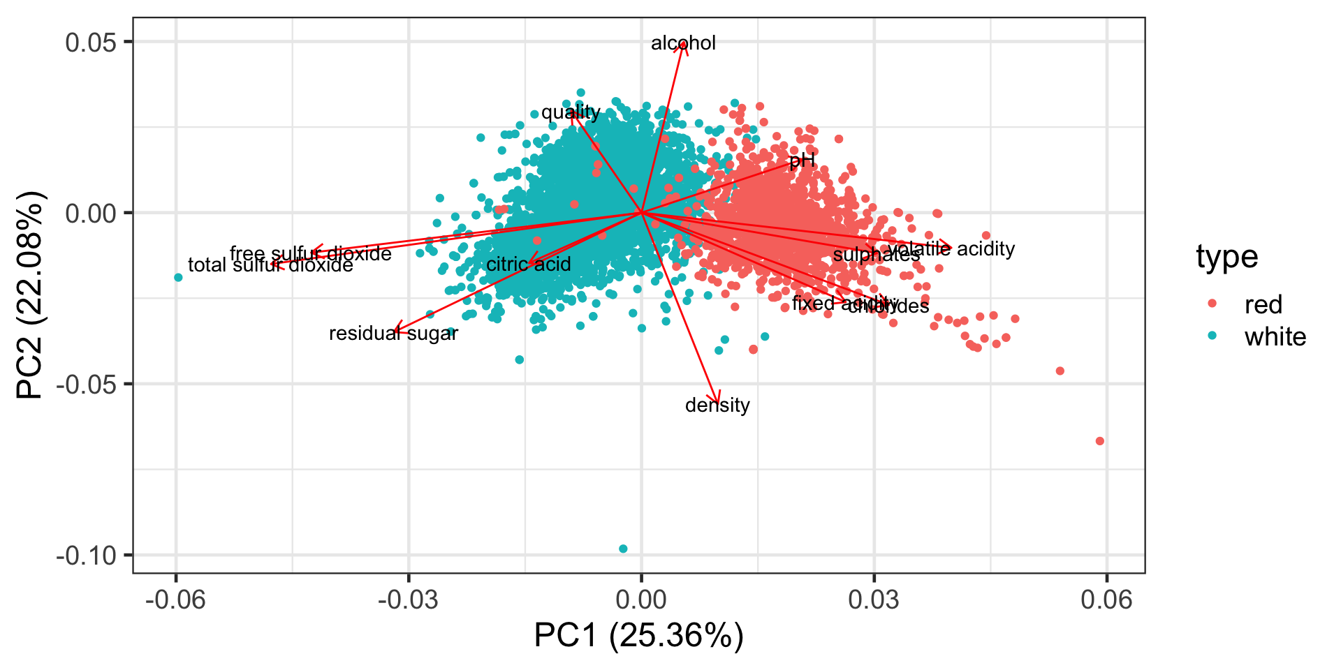
Correlation biplot
Distance biplot
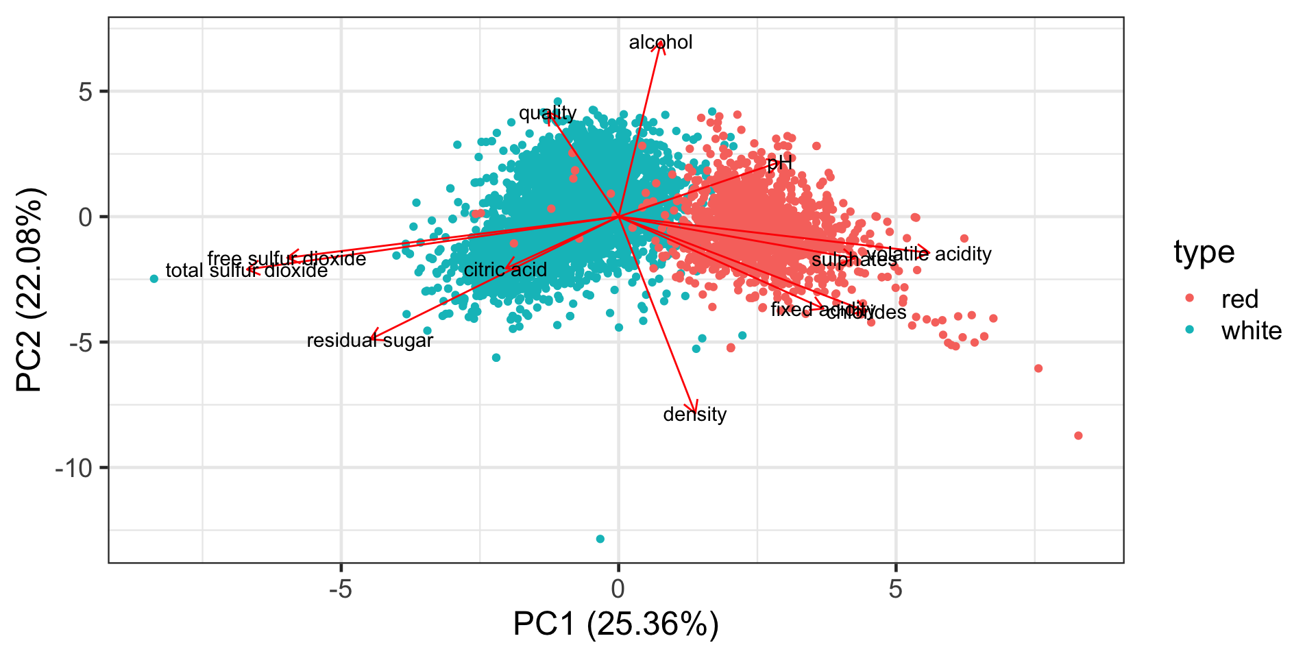
Interpreting a biplot
- The distance between observations implies similarity between observations.
- The angles between variables tell us something about correlation (approximately)
- citric acid and residual sugar are highly positively correlated as the angle between them is close to zero.
- quality and pH are close to uncorrelated as the angle between them is close 90 degrees.
- pH and citric acid are highly negatively correlated as the angle between them is close to 180 degrees.
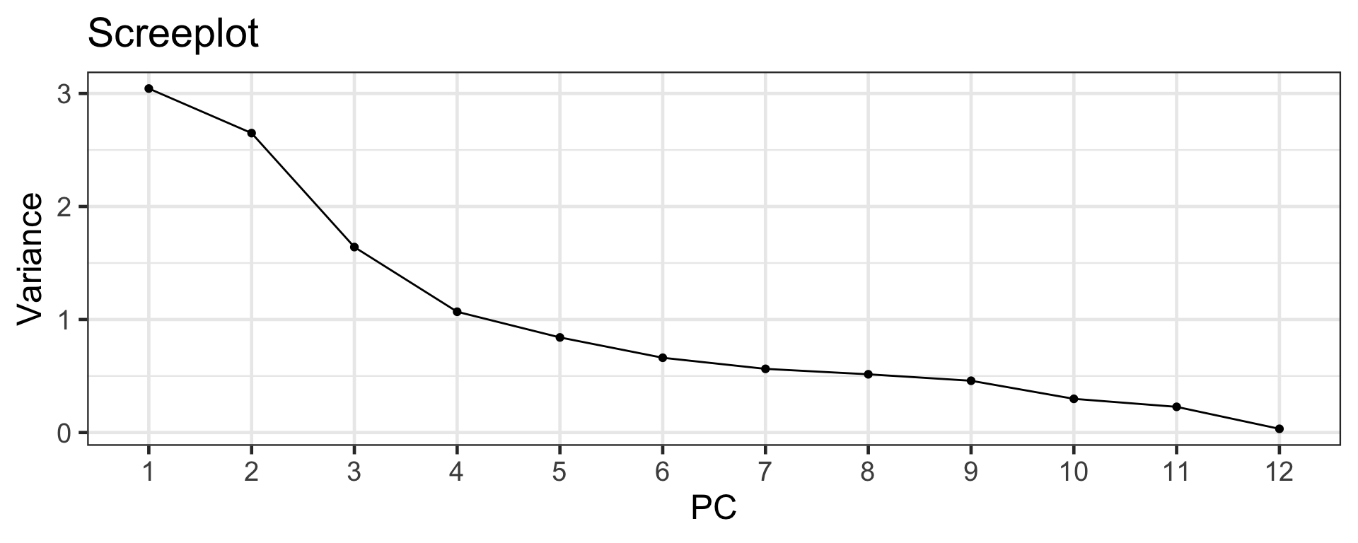
Scree plot
Selecting the number of principal components
Elbow method
- The scree plot can be used to select the number of PCs.
- Look for the “elbow” of the scree plot (around 4-6).
- There is some subjectiveness to the selection!

Kaiser’s rule
- Kaiser’s rule states to select all PCs with a variance greater than 1.
Importance of components:
                          PC1    PC2    PC3     PC4     PC5     PC6     PC7
Standard deviation     1.7445 1.6276 1.2810 1.03370 0.91728 0.81338 0.75056
Proportion of Variance 0.2536 0.2208 0.1367 0.08905 0.07012 0.05513 0.04695
Cumulative Proportion  0.2536 0.4744 0.6111 0.70016 0.77028 0.82541 0.87236
                           PC8     PC9    PC10    PC11    PC12
Standard deviation     0.71786 0.67689 0.54605 0.47678 0.18089
Proportion of Variance 0.04294 0.03818 0.02485 0.01894 0.00273
Cumulative Proportion 0.91530 0.95348 0.97833 0.99727 1.00000- Here we select 4 PCs.
Interpreting PCs
- Remember that PCs do nothing more than finding uncorrelated linear combinations of the variables that explain the variance of the data.
- It can be incredibly useful to find the interpretation of PCs but this relies on the context of data.
Multi-dimensional scaling
Motivation
- Suppose we have n observations and p (numerical) variables.
- When p = 2, we can easily draw a scatterplot to see the disances between observations.
- However, when p > 2 then there isn’t an easy way to visualise the distances between observations.
- But, we can get a close approximation of the distances using multi-dimensional scaling (MDS) by finding a low (usually two) dimensional represenation of pairwise distances between observations.
Classical MDS
Dwinec <- winec %>%
# note that we are removing the categorical variable `type` here!
select(-type) %>%
# then standardising the data
scale() %>%
# and calculating the distances between observations (ED is default)
dist()
# add the row labels back
attributes(Dwinec)$Labels <- winec$type
# perform the classical (metric) MDS
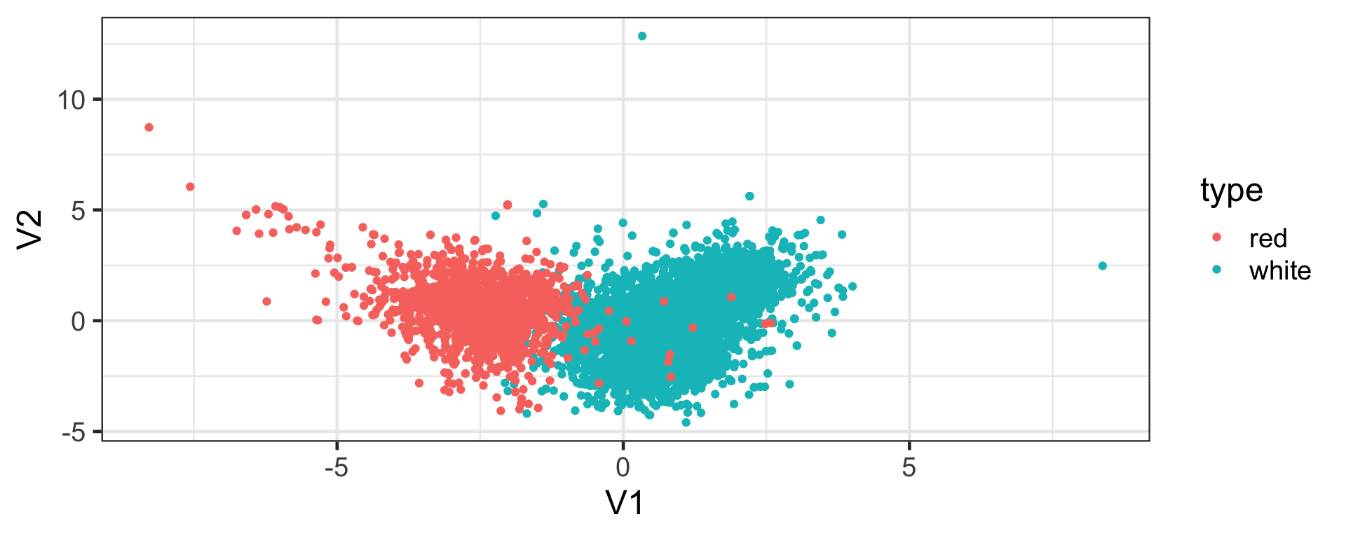
mdsout <- cmdscale(Dwinec, k = 2)
head(mdsout) [,1] [,2]
white 2.49817594 3.1644222
white -0.08269114 -0.4738874
white 0.18302503 0.2916830
white 1.75126084 0.7336440
white 1.75126084 0.7336440
white 0.18302503 0.2916830Visualising the MDS output
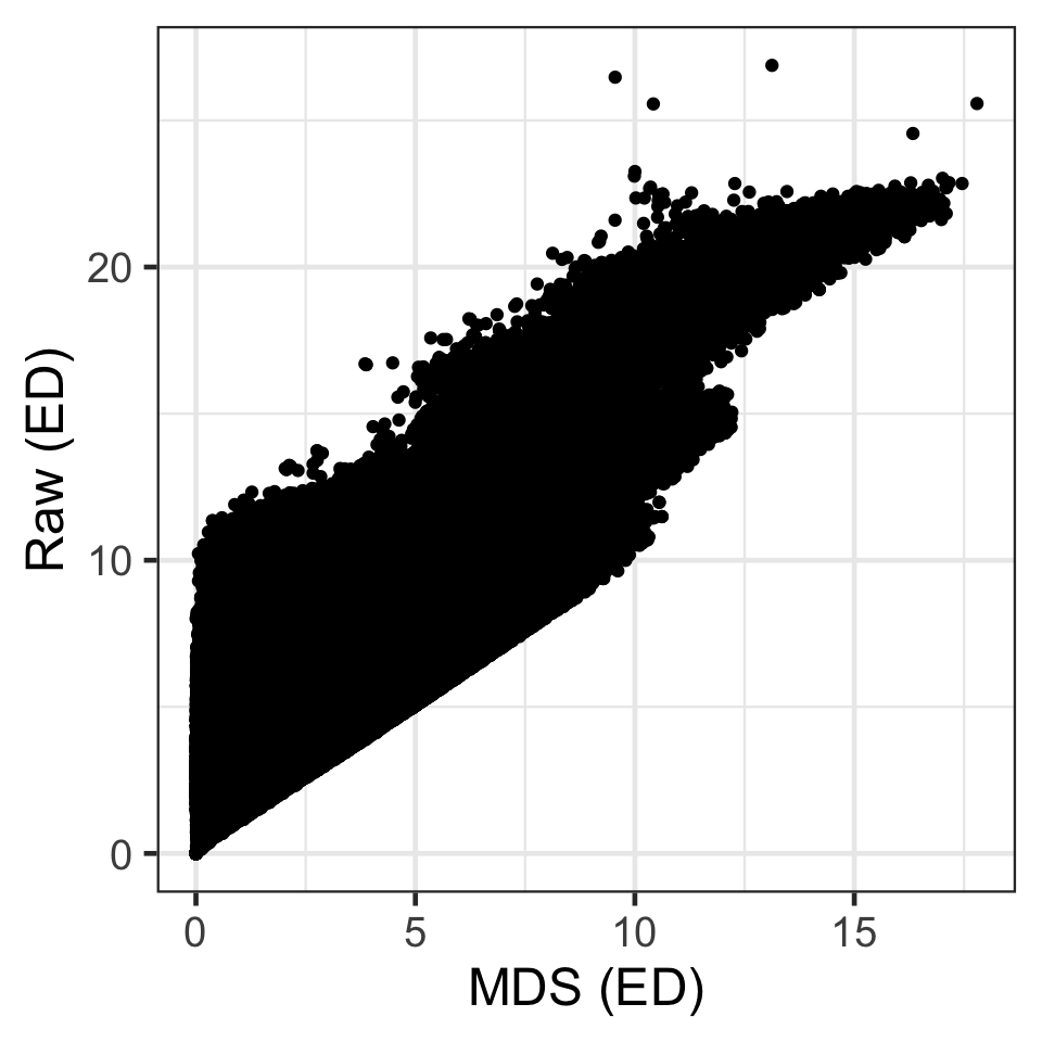
Distances
D_{Euclidean}(\boldsymbol{x}_i, \boldsymbol{x}_j) = \sqrt{\sum_{s = 1}^p (x_{is} - x_{js})^2}.
- So for example, D_{Euclidean}(\boldsymbol{x}_1, \boldsymbol{x}_2) = 5.415.
- But for D_{Euclidean}(\boldsymbol{z}_1, \boldsymbol{z}_2) = \sqrt{(2.498 - (-0.083))^2 + (3.164 - (-0.474))^2} = 4.461.
- Another example, D_{Euclidean}(\boldsymbol{x}_1, \boldsymbol{x}_3) = 4.392.
- But D_{Euclidean}(\boldsymbol{z}_1, \boldsymbol{z}_2) = \sqrt{(2.498 - 0.183)^2 + (3.164 - 0.292)^2} = 3.69.
Comparing raw and MDS distances
Classical MDS
- In classical MDS, the aim is to minimise the strain function:
\text{Strain} = \sum_{i=1}^{n-1}\sum_{j>i}\left(D(\boldsymbol{x}_i, \boldsymbol{x}_j) - D(\boldsymbol{z}_i, \boldsymbol{z}_j)\right)^2.
- The above has a tractable solution when Euclidean distance is used.
- The solution rotates the points until the 2D projection is close to the input distances.
Sammon mapping
- An alternative objective is to minimise the stress function:
\text{Stress} = \sum_{i=1}^{n-1}\sum_{j>i}\frac{\left(D(\boldsymbol{x}_i, \boldsymbol{x}_j) - D(\boldsymbol{z}_i, \boldsymbol{z}_j)\right)^2}{D(\boldsymbol{x}_i, \boldsymbol{x}_j)}.
- This ensures that points that observations with small distances are close to in the MDS output as well, preserving the local structure.
- This is refererd to as sammon mapping.
Modern MDS
- Methods for finding a low dimensional representation of high dimensional data are more recently referred to as manifold learning.
- Low-dimensional representations can also be used as features downstream in classification or regression problems.
- Some of these examples include,
- Local linear embeddings (LLE)
- IsoMap
- t-SNE
- UMAP, and so on.
Takeaways
- Principal components are linear combination of the data variables.
- Multi-dimensional scaling is a non-linear dimensionality reduction.
- They both present low-dimenstional representation of the full data and useful for downstream analysis.

ETC3250/5250 Week 8