Ensemble methods combine predictions from multiple models.
The idea is that the combining results from multiple models can (but not always) result in a better predictive performance than a single model by “averaging out” the individual weaknesses (i.e. errors).
These aggregation generally reduces the variance.
However, the aggregation process often loses the interpretation of the single models.
Tree ensemble methods
Some well-known tree ensemble methods include:
Bagging: combining predictions based on bootstrap samples.
Random forests: combining predictions based on bagging and random subset selection of predictors.
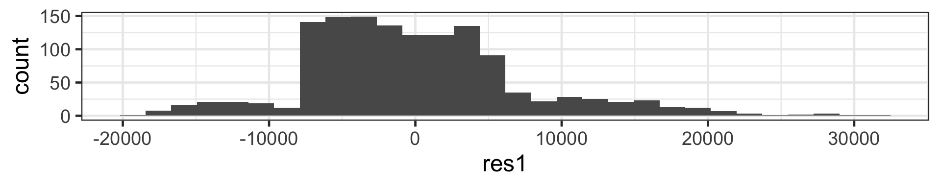
Boosting: combining predictions from models sequentially fit to residuals from previous fit.
Bagging
Bagging ensemble learning
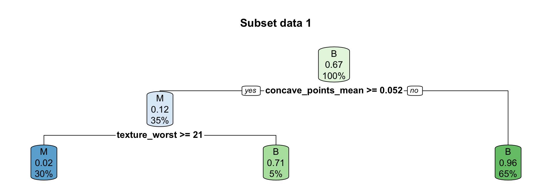
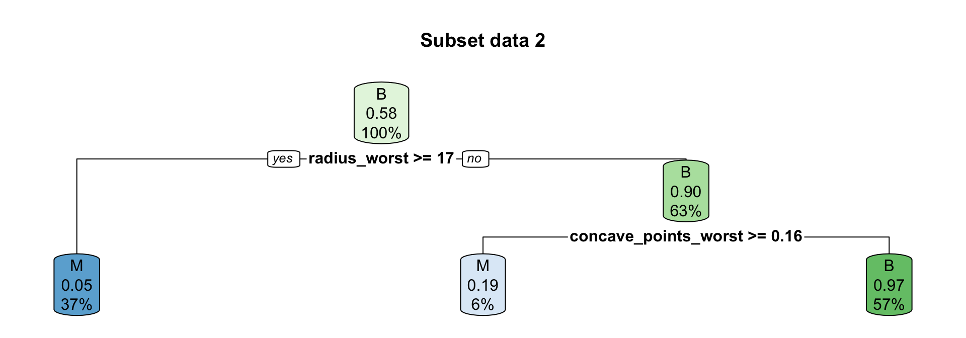
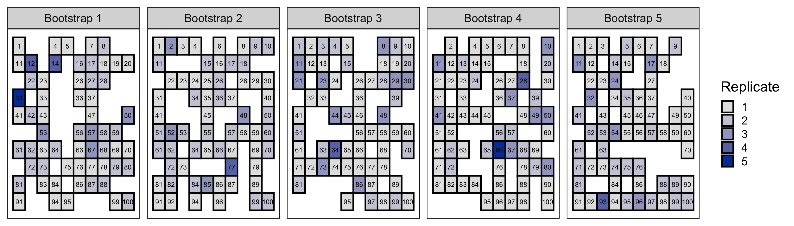
Bootstrap aggregating, or bagging for short, is an ensemble learning method that combines predictions from trees to bootstrapped data.
Recall boostrap involves resampling observations with replacement.
Random forests build an ensemble of deep independent trees.
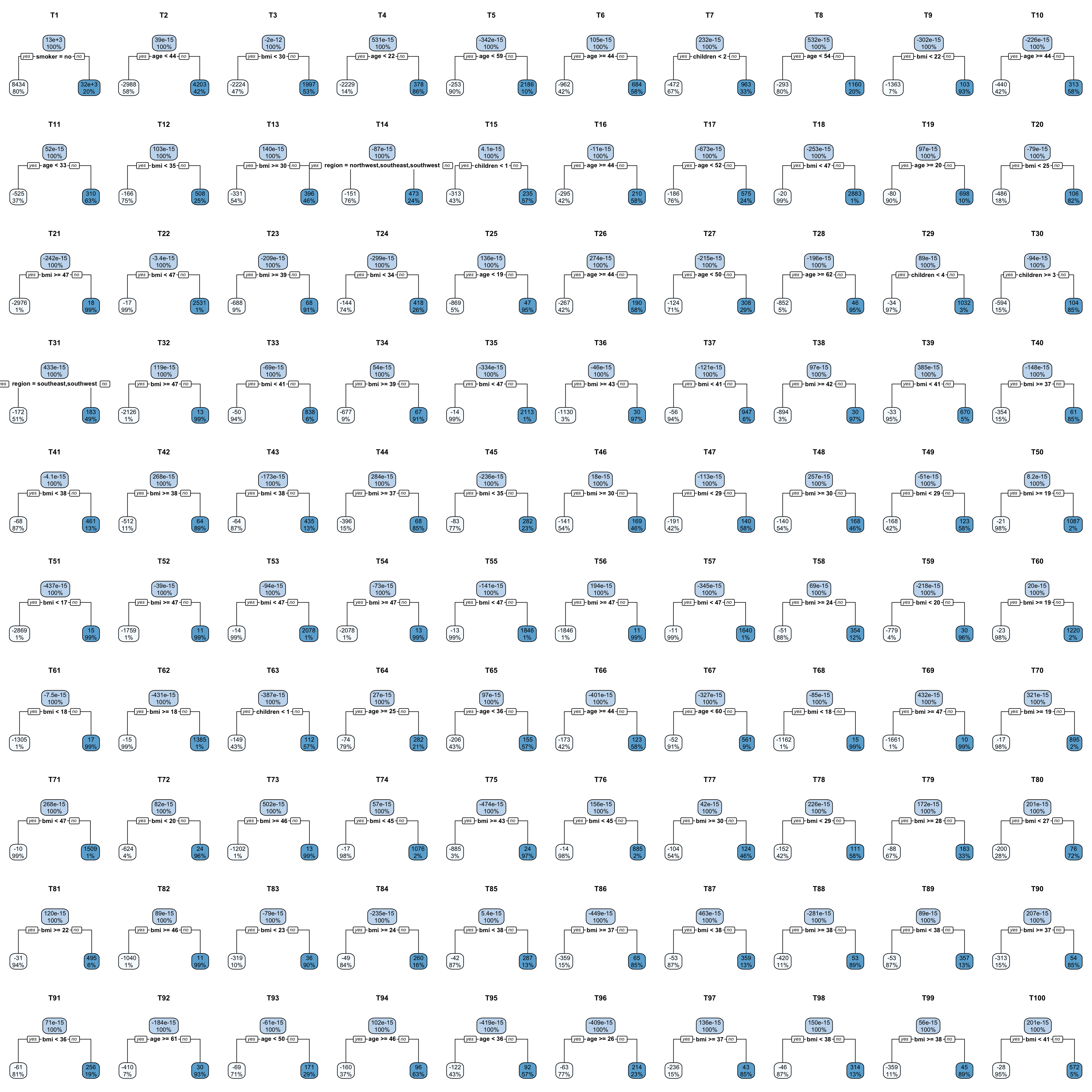
Boosted trees build an ensemble of shallow trees in sequence with each tree learning and improving on the previous one.
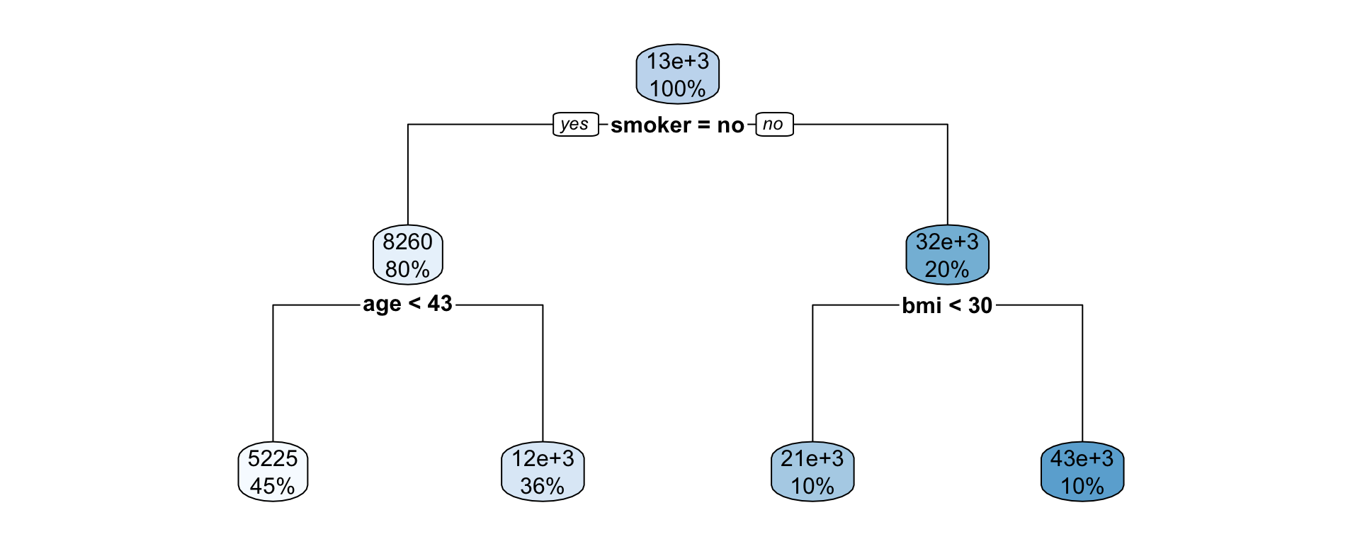
Boosting for regression trees first tree
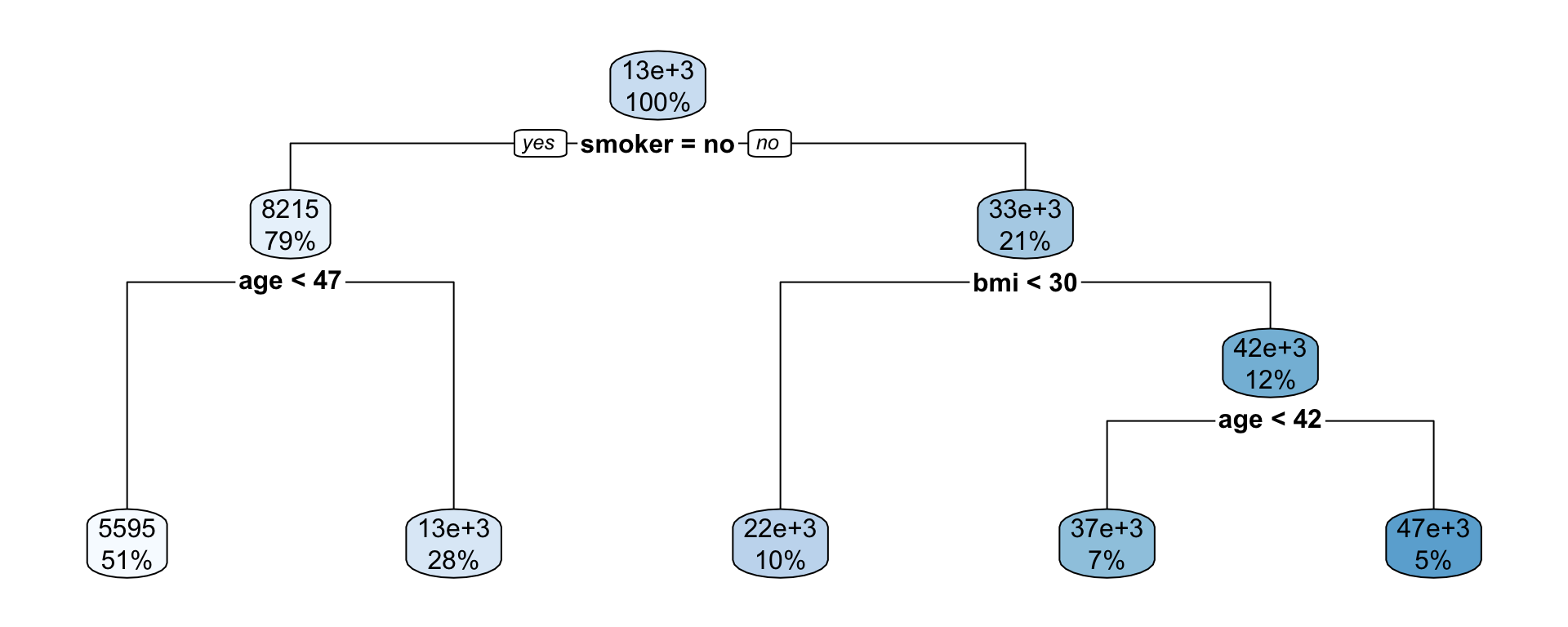
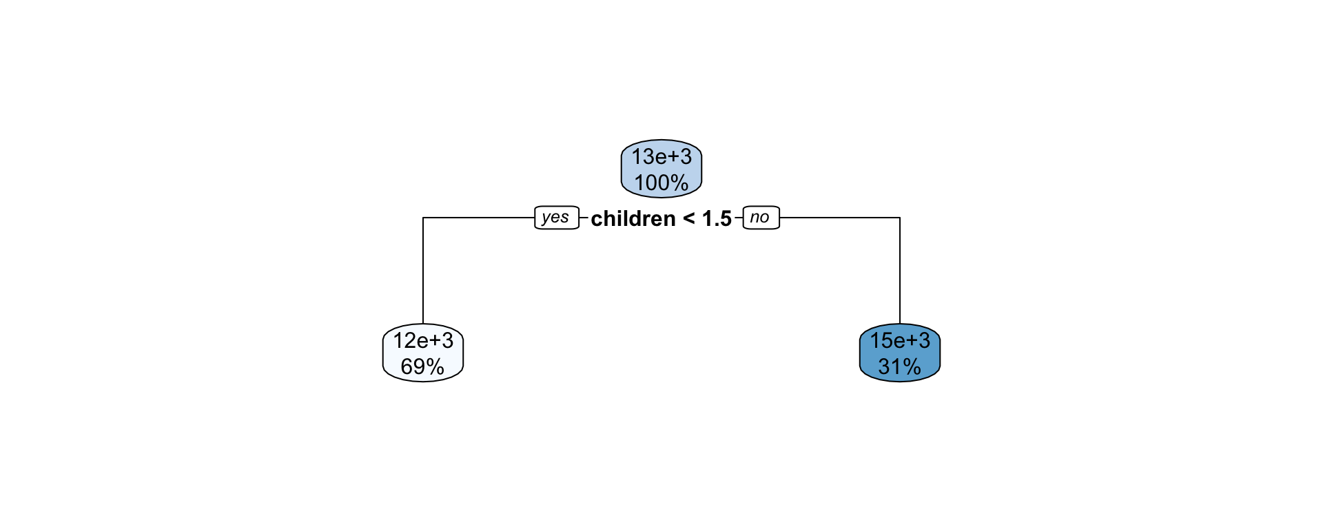
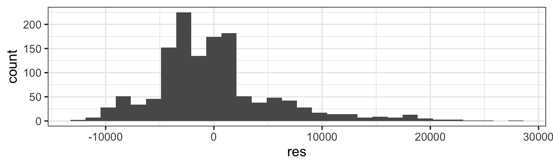
Suppose we fit a (shallow) regression tree, T^1, to y_1, y_2, \dots, y_n for the set of predictors \boldsymbol{x}_1, \boldsymbol{x}_2, \dots, \boldsymbol{x}_p.
We then use r_1^1, r_2^1, \dots, r_n^1 as your “response” data to fit the next tree, T^2, using the same set of predictors \boldsymbol{x}_1, \boldsymbol{x}_2, \dots, \boldsymbol{x}_p.
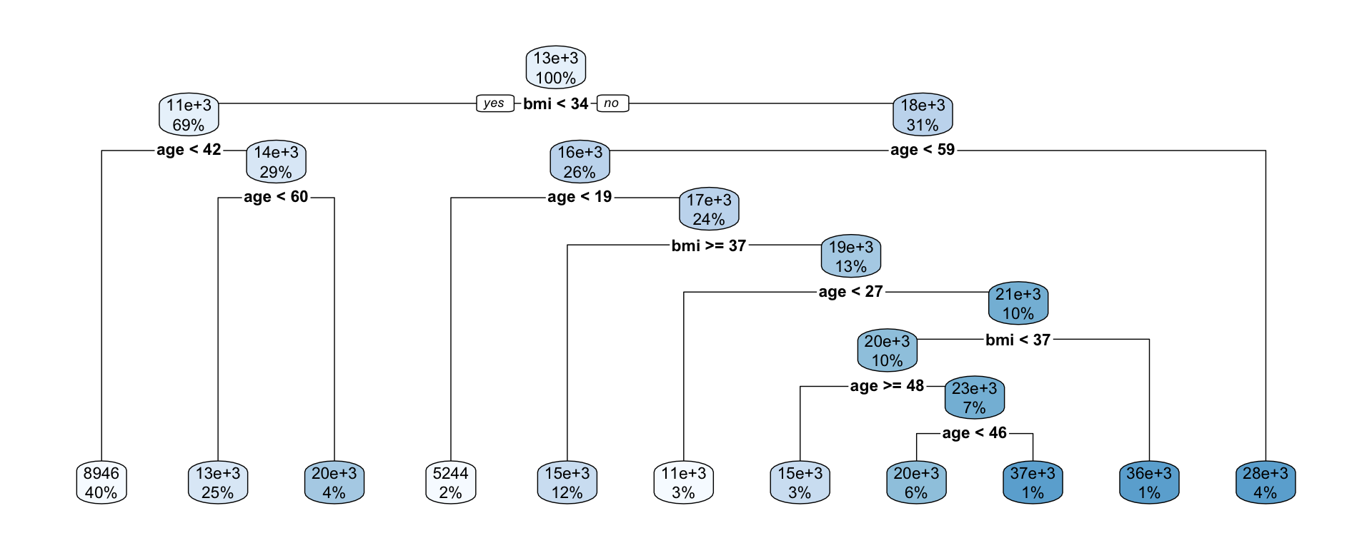
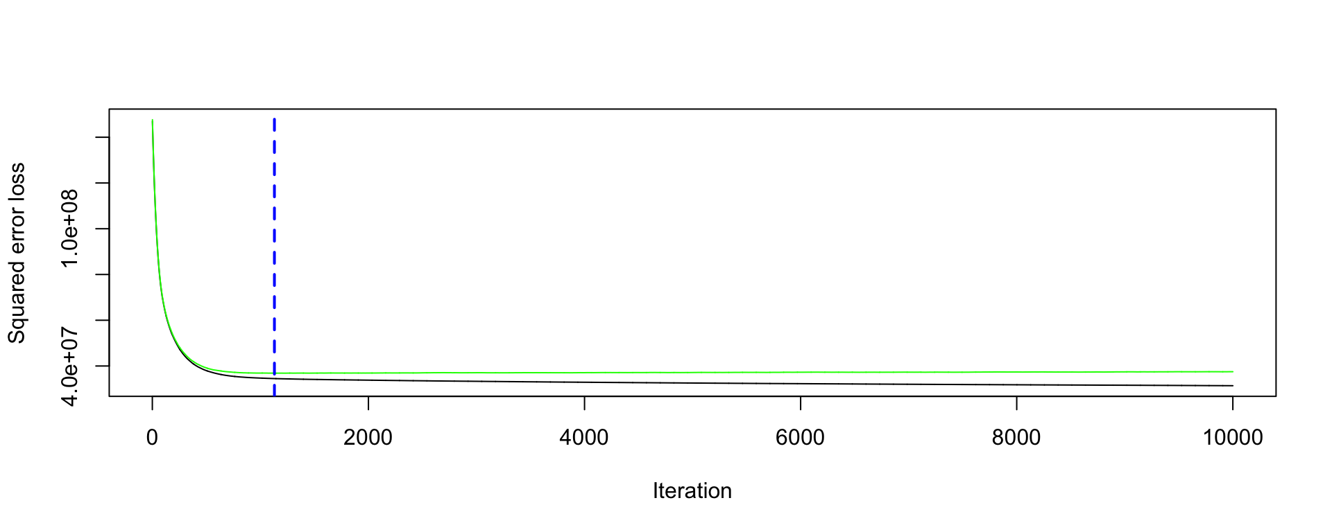
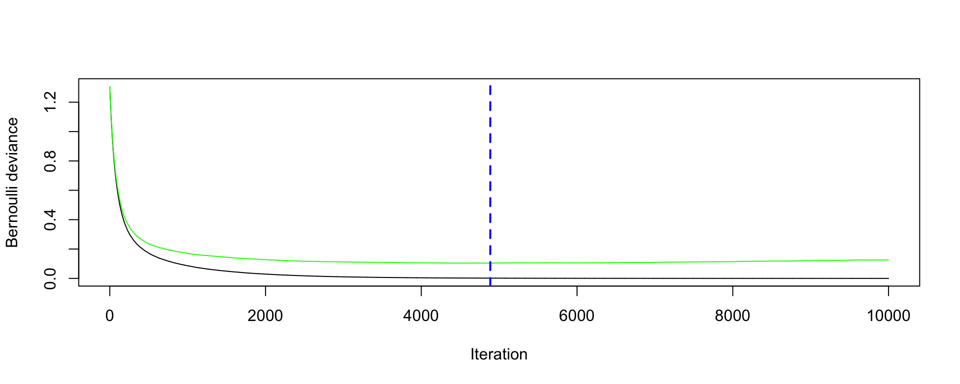
Each iteration (tree) increases accuracy a little but too many iterations result in overfitting.
Smaller \lambda slows the learning rate.
Each tree is shallow – if the tree has only one split, it is called a stump.
Other ensemble tree methods
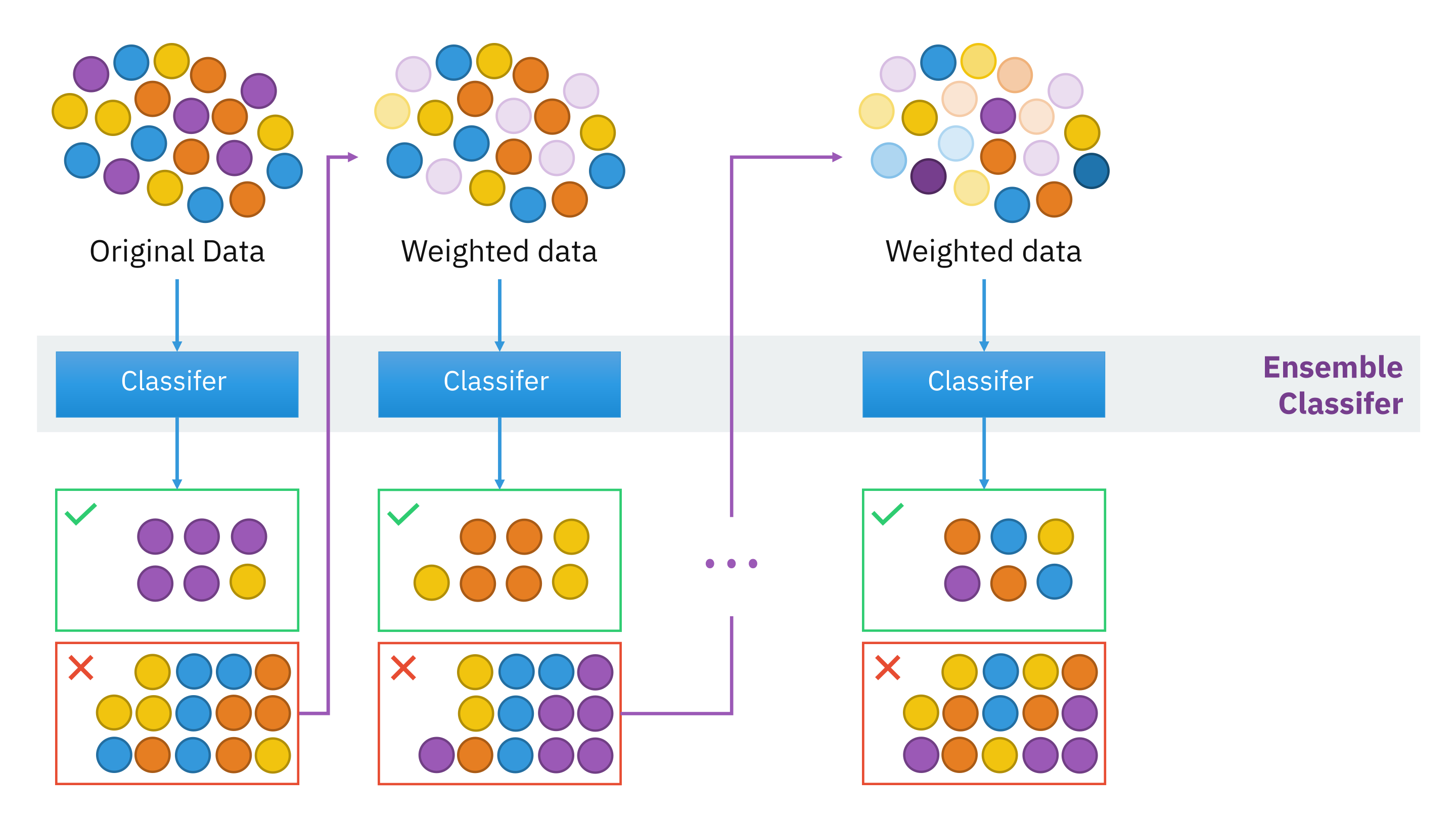
Adaptive boosting
Adaptive boosting, or AdaBoost, is a type of boosting method where data for successive iterations of trees are based on weighted data.
There is a higher weight put on observations that were wrongly classified or has large error.
AdaBoost can be considered as a special case of (extreme) gradient boosting.
Gradient boosting
Gradient boosting involves a loss function, L(y_i|f_m) where \hat{y}_i^m = f_m(\boldsymbol{x}_i|T^m).
The choice of the loss function depends on the context, e.g. sum of the squared error may be used for regression problems and logarithmic loss function is used for classification problems.
The loss function must be differentiable.
Compute the residuals as r_i^m = - \frac{\partial L(y_i|f_m(\boldsymbol{x}_i))}{\partial f_m(\boldsymbol{x}_i)}.
Extreme gradient boosting
Extreme gradient boosted trees, or XGBoost, makes improvements to gradient boosting algorithms.
XGBoost implements many optimisation methods that allow for computationally fast fit of the model (e.g. parallelised tree building, cache awareness computing, efficient handling of missing data).
XGBoost also implements algorithmic techniques to ensure better model fit (e.g. regularisation to avoid overfitting, in-build cross-validation, pruning trees based on depth-first approach).
Combining predictions
Business decisions
Suppose a corporation needs to make a decision, e.g. deciding
between strategy A, B or C (classification problem) or
how much to spend (regression problem).
An executive board is presented with recommendations from experts.
Experts
👨✈️
🕵️♀️
🧑🎨
🧑🎤
🧑💻
👷
👨🔧
Classification
A
B
C
B
A
C
B
Regression
$9.3M
$9.2M
$8.9M
$3.1M
$9.2M
$8.9M
$9.4M
What would your final decision be for each problem?
Ensemble learning
Experts
👨✈️
🕵️♀️
🧑🎨
🧑🎤
🧑💻
👷
👨🔧
Classification
A
B
C
B
A
C
B
Regression
$9.3M
$9.2M
$8.9M
$3.1M
$9.2M
$8.9M
$9.4M
Combining predictions from multiple models depends on whether you have a regression or classification problem.
The simplest approach for:
regression problems is to take the average ($8.1M here), and
classification problems is to take the majority vote (B here).