ETC3250/5250

Introduction to Machine Learning

Discriminant analysis

Lecturer: Emi Tanaka

Department of Econometrics and Business Statistics

Discriminant analysis

  • Another approach for building a classification model is with discriminant analysis (DA).
  • There are two main approaches we cover in this unit:
    • linear discriminant analysis (LDA), and
    • quadratic discriminant analysis (QDA).

Logistic regression vs LDA vs QDA

  • For DA, we estimate P(X|Y) shown as the contours to deduce P(Y|X) used to get the decision boundary.

DA in a nutshell

  • DA involves assuming that the distribution of the predictors has a multivariate Normal distribution:
    • \boldsymbol{X}_{k} \sim N(\boldsymbol{\mu}_{k}, \mathbf{\Sigma}_k) for class k = 1, \dots, K where
      • \boldsymbol{\mu}_{k} is the p-vector of means, and
      • \mathbf{\Sigma}_k is the p\times p variance-covariance matrix for the j-th predictor.
  • DA provides a low-dimensional projection of the p-dimensional space, where the class means \boldsymbol{\mu}_{k} are the most separated relative to the variance-covariance \mathbf{\Sigma}_k.

Background

Bayes theorem

  • Let f_k(x) be the density function for predictor x for class k.
  • Bayes theorem (for K classes) states that the posterior probability: P(Y = k|X = x) = p_k(x) = \frac{\pi_kf_k(x)}{\sum_{k=1}^K \pi_kf_k(x)} where \pi_k = P(Y = k) is the prior probability that the observation comes from class k.

Univariate Normal (Gaussian) distribution

f(x) = \frac{1}{\sqrt{2 \pi} \sigma} \text{exp}~ \left( - \frac{1}{2 \sigma^2} (x - \mu)^2 \right).

Code
tibble(x = seq(-5, 7, length = 100)) %>% 
  mutate(f1 = dnorm(x, 2, 1),
         f2 = dnorm(x, -1, 1),
         f3 = dnorm(x, 3, 2)) %>% 
  pivot_longer(f1:f3, values_to = "f") %>% 
  ggplot(aes(x, f)) + 
  geom_line(aes(color = name), linewidth = 1.2) +
  labs(y = "f(x)", color = "") +
  scale_color_discrete(labels = c("N(2, 1)", "N(-1, 1)", "N(3, 4)"))

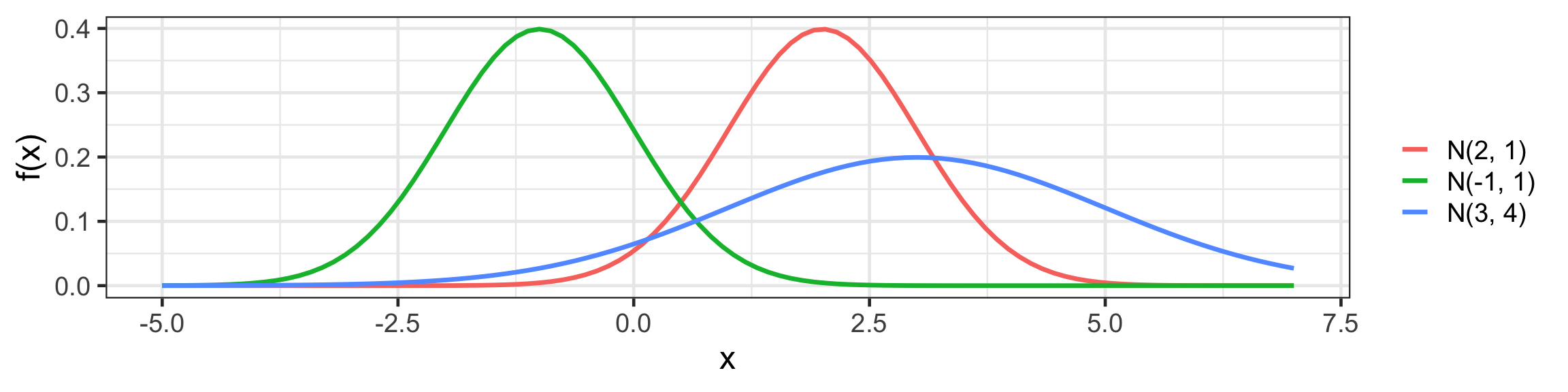
Multivariate Normal (Gaussian) distribution

f(\boldsymbol{x}) = \frac{1}{(2\pi)^{\frac{p}{2}}|\mathbf{\Sigma}|^{\frac{1}{2}}} \exp\left(-\frac{1}{2}(\boldsymbol{x}-\boldsymbol{\mu})^\top\mathbf{\Sigma}^{-1}(\boldsymbol{x}-\boldsymbol{\mu})\right)

  • \boldsymbol{\mu} is a p-vector of means, and
  • \mathbf{\Sigma} is a p\times p variance-covariance matrix.


Code
expand_grid(x1 = seq(-5, 5, length = 100),
            x2 = seq(-5, 5, length = 100)) %>% 
  rowwise() %>% 
  mutate(f1 = mvtnorm::dmvnorm(c(x1, x2), mean = c(2, 1), sigma = matrix(c(1, 0.5, 0.5, 1), 2, 2)),
         f2 = mvtnorm::dmvnorm(c(x1, x2), mean = c(1, 2), sigma = matrix(c(1, 0, 0, 1), 2, 2)),,
         f3 = mvtnorm::dmvnorm(c(x1, x2), mean = c(-1, 1), sigma = matrix(c(2, 0.5, 0.5, 1), 2, 2)),) %>% 
  pivot_longer(f1:f3, values_to = "f") %>% 
  ggplot(aes(x1, x2, z = f)) + 
  geom_contour(aes(color = name), linewidth = 1.2) +
  labs(color = "") +
  guides(color = "none")
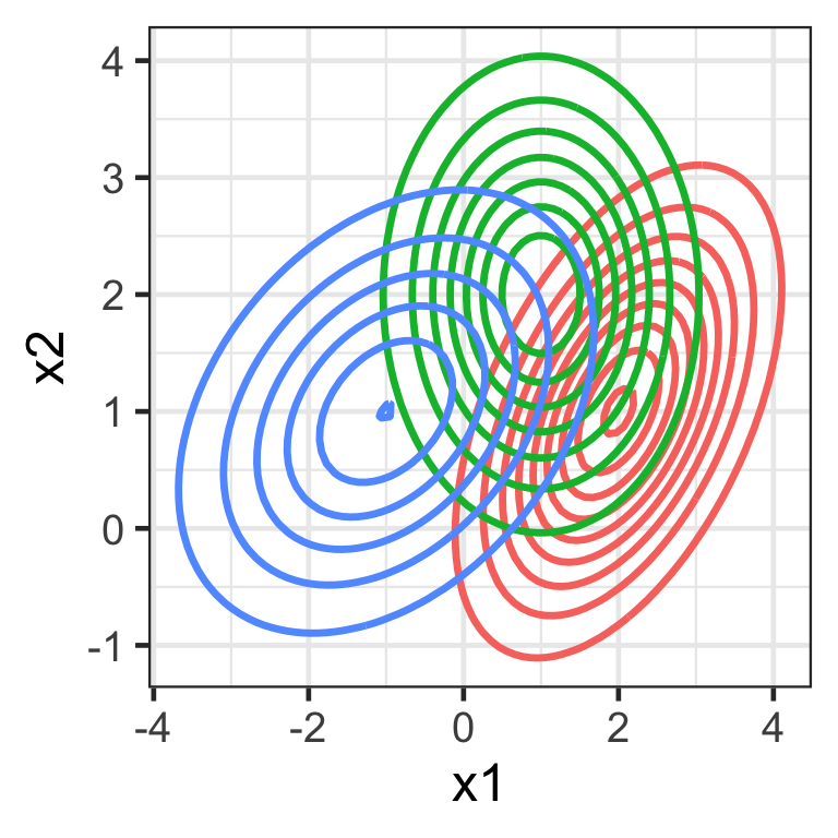
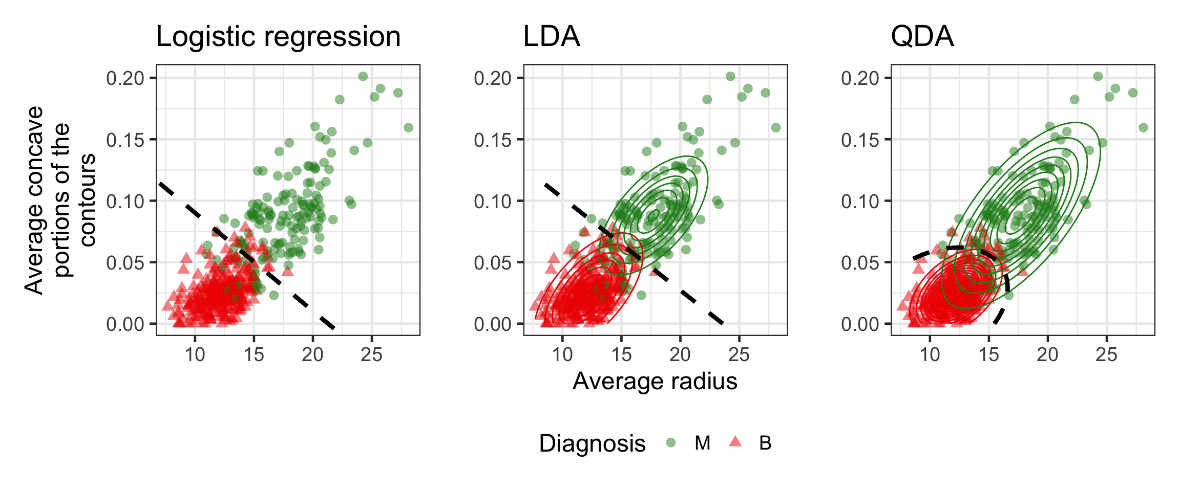
Linear Discriminant Analysis

LDA

  • Recall, we assume that \boldsymbol{X}_{k} \sim N(\boldsymbol{\mu}_{k}, \mathbf{\Sigma}_k) for k = 1, \dots, K.

  • In LDA, we further assume that \mathbf{\Sigma}_1 = \mathbf{\Sigma}_2 = \dots = \mathbf{\Sigma}_k = \mathbf{\Sigma}.

  • Then by Bayes theorem, the posterior is given as: p_k(\boldsymbol{x}) = \frac{\pi_k\exp~ \left( - \frac{1}{2} (\boldsymbol{x} - \boldsymbol{\mu}_k)\mathbf{\Sigma}^{-1}(\boldsymbol{x} - \boldsymbol{\mu}_k) \right) }{ \sum_{k = 1}^K \pi_k \exp~ \left( - \frac{1}{2} (\boldsymbol{x} - \boldsymbol{\mu}_k)\mathbf{\Sigma}^{-1}(\boldsymbol{x} - \boldsymbol{\mu}_k) \right) }.

  • We assign new observation \boldsymbol{X} = \boldsymbol{x}_0 to the class with the highest p_k(\boldsymbol{x}_0), referred to as the maximum a posteriori estimation (MAP).

LDA with R: \boldsymbol{\mu}_k

  • The LDA model can be fit using lda() via the maximum likelihood estimate in the MASS package as:
cancer_lda <- MASS::lda(diagnosis ~ radius_mean + concave_points_mean, 
                        data = cancer_train, 
                        method = "mle")
  • The estimate of \begin{bmatrix}\boldsymbol{\mu}_{\text{A}}^\top\\ \boldsymbol{\mu}_{\text{B}}^\top \end{bmatrix} is found:
cancer_lda$means
  radius_mean concave_points_mean
M    17.71993          0.08796497
B    12.20888          0.02551768

LDA with R: \mathbf{\Sigma}

  • The estimate of \mathbf{\Sigma} is found:
cancer_lda_sigma <- cancer_train %>% 
  # first center predictors based on MLE of class means
  mutate(x1 = radius_mean - cancer_lda$means[diagnosis, "radius_mean"],
         x2 = concave_points_mean - cancer_lda$means[diagnosis, "concave_points_mean"]) %>% 
  select(x1, x2) %>% 
  # find the sample variance-covariance matrix
  var()

cancer_lda_sigma
           x1           x2
x1 5.39571618 0.0348868055
x2 0.03488681 0.0005928822

Quadratic Discriminant Analysis

QDA with R: \boldsymbol{\mu}_k

  • The QDA model can be fit using qda() via the maximum likelihood estimate in the MASS package as:
cancer_qda <- MASS::qda(diagnosis ~ radius_mean + concave_points_mean, 
                        data = cancer_train, 
                        method = "mle")
  • The estimate of \begin{bmatrix}\boldsymbol{\mu}_{\text{A}}^\top\\ \boldsymbol{\mu}_{\text{B}}^\top \end{bmatrix} is found:
cancer_qda$means
  radius_mean concave_points_mean
M    17.71993          0.08796497
B    12.20888          0.02551768

QDA with R: \mathbf{\Sigma}

  • The estimate of \mathbf{\Sigma} is found:
cancer_qda_sigma <- cancer_train %>% 
  # first center predictors based on MLE of class means
  mutate(x1 = radius_mean - cancer_qda$means[diagnosis, "radius_mean"],
         x2 = concave_points_mean - cancer_qda$means[diagnosis, "concave_points_mean"]) %>% 
  group_by(diagnosis) %>% 
  summarise(sigma = list(var(data.frame(x1, x2))))


cancer_qda_sigma$sigma[[1]]
           x1          x2
x1 9.91949800 0.076928052
x2 0.07692805 0.001252928
cancer_qda_sigma$sigma[[2]]
           x1          x2
x1 2.93888569 0.011998849
x2 0.01199885 0.000233707

Predictions from dicriminant models

library(MASS)
qthresh <- 0.5
cancer_pred <- cancer_test %>% 
  mutate(prob_lda = predict(cancer_lda, .)$posterior[, 1],
         prob_qda = predict(cancer_qda, .)$posterior[, 1],
         pred_lda = factor(ifelse(prob_lda > qthresh, "M", "B"), levels = c("M", "B")),
         pred_qda = factor(ifelse(prob_qda > qthresh, "M", "B"), levels = c("M", "B"))) %>% 
  select(prob_lda, prob_qda, pred_lda, pred_qda, diagnosis)

cancer_pred
# A tibble: 142 × 5
   prob_lda prob_qda pred_lda pred_qda diagnosis
      <dbl>    <dbl> <fct>    <fct>    <fct>    
 1    0.730    1.00  M        M        M        
 2    0.446    0.981 B        M        M        
 3    0.257    0.471 B        B        M        
 4    0.733    0.999 M        M        M        
 5    0.149    0.340 B        B        M        
 6    0.997    1.00  M        M        M        
 7    0.608    0.977 M        M        M        
 8    0.257    0.357 B        B        M        
 9    0.115    0.155 B        B        B        
10    0.993    1.00  M        M        M        
# … with 132 more rows

Classification metrics

library(yardstick)
cancer_pred %>% 
  pivot_longer(-diagnosis, names_to = c(".value", "model"), names_sep = "_") %>% 
  group_by(model) %>% 
  metric_set(sensitivity, specificity, precision, recall, pr_auc, roc_auc, 
             f_meas, accuracy, bal_accuracy, kap, mcc, ppv, npv, j_index)(., 
                                                   truth = diagnosis, 
                                                   prob, 
                                                   estimate = pred) %>% 
  pivot_wider(.metric, names_from = model, values_from = .estimate) %>% 
  mutate(winner = ifelse(lda > qda, "lda", "qda"))
# A tibble: 14 × 4
   .metric        lda   qda winner
   <chr>        <dbl> <dbl> <chr> 
 1 sensitivity  0.738 0.852 qda   
 2 specificity  0.988 0.914 lda   
 3 precision    0.978 0.881 lda   
 4 recall       0.738 0.852 qda   
 5 f_meas       0.841 0.867 qda   
 6 accuracy     0.880 0.887 qda   
 7 bal_accuracy 0.863 0.883 qda   
 8 kap          0.748 0.769 qda   
 9 mcc          0.767 0.769 qda   
10 ppv          0.978 0.881 lda   
11 npv          0.833 0.892 qda   
12 j_index      0.725 0.766 qda   
13 pr_auc       0.969 0.958 lda   
14 roc_auc      0.977 0.967 lda   

Takeaways

Logistic regression

  • Goal: directly estimate P(Y \lvert X)
  • Assumptions: no assumptions on predictor space

Discriminant analysis

  • Goal: estimate P(X \lvert Y) to then deduce P(Y \lvert X)
  • Assumptions: predictors are normally distributed