ETC3250/5250
Introduction to Machine Learning
Regularisation
Lecturer: Emi Tanaka
Department of Econometrics and Business Statistics
Too many predictors
- Subset selection methods are a useful way of selecting important predictors.
- However, they
- are not guaranteed to provide the best model,
- can be slow to compute if \(p\) is large, and
- have issues when \(p > n\).
- Regularisation (shrinkage) methods avoid these issues.
Ordinary least squares
- OLS fits the coefficients as \[\hat{\boldsymbol\beta}= \underset{\boldsymbol\beta\in\mathbb{R}^{p+1}}{\mbox{arg min}}\ \sum_{i = 1}^n \left(y_i - \beta_0 - \sum_{j = 1}^p \beta_j x_{ij} \right)^2 = \underset{\boldsymbol\beta\in\mathbb{R}^{p+1}}{\mbox{arg min}}~\text{RSS}(\boldsymbol{\beta}).\]
- This is an unconstrained optimization problem.
Visualising the RSS
\[y_i = \beta_1x_{i1} + \beta_2x_{i2} + e_i,\]
Data simulated with: \(\beta_1 = 2, \beta_2 = 3, e_i \sim N(0, 1)\)
Axis grid
X: \(\beta_1\)Y: \(\beta_2\)Z: \(\text{RSS}(\beta_1, \beta_2)\)
Shrinkage methods
- Shrinkage methods fit a model containing all \(p\) predictors using a technique that constrains or regularizes the coefficient estimates.
- This shrinks some of the coefficient estimates towards zero.
- There are three main methods:
- Ridge regression (also called L2 regularisation)
- Lasso (also called L1 regularisation)
- Elastic net (linear combination of L1 and L2 regularisation)
Ridge regression
Ridge regression
- Ridge regression is similar to except with constraint:
\[{\hat{\boldsymbol\beta}_{ridge} = \underset{\boldsymbol\beta\in\mathbb{R}^{p+1}}{\mbox{arg min}}\ \text{RSS}(\boldsymbol{\beta})} \color{#006DAE}{\quad {\text{subject to } \sum_{j=1}^p\beta_j^2\leq s}}.\]
- \(s\) bounds the magnitude of the coefficients.
- If \(s = 0\), then \(\beta_1, \dots, \beta_p\) are equal to zero.
- If \(s = \infty\), then ridge regression = OLS.
Shrinkage for ridge regression
\[\sum_{j=1}^p\beta_j^2\leq s\]
- Think of \(s\) as a budget - we allocate \(s\) to \(p\) predictors.
- Important predictors get a big part of the budget.
- In this formulation, \(\beta_j\) is shrunk towards zero (if the intercept is fitted into the model) but never actually zero.
- Shrinkage is not applied to the intercept coefficient.
Visualising the ridge regression constraint
\(\beta_1^2 + \beta_2^2 \leq 1\)
Axis grid
X: \(\beta_1\)Y: \(\beta_2\)Z: \(\text{RSS}(\beta_1, \beta_2)\)
Visualising the ridge regression
\[{\hat{\boldsymbol\beta} = \underset{\boldsymbol\beta\in\mathbb{R}^{2}}{\mbox{arg min}}\ \text{RSS}(\boldsymbol{\beta})}\]
\[\text{subject to } \beta_1^2 + \beta_2^2\leq s\]
- Axis grid
X: \(\beta_1\)Y: \(\beta_2\)Z: \(\text{RSS}(\beta_1, \beta_2)\)
Lagrange function
Constrained optimization problems are much harder than unconstrained ones.
Finding points in one surface is much easier than finding points simultaneously on both surfaces.
Ridge regression can be re-written as a Lagrange function: \[\hat{\boldsymbol\beta}_{\text{ridge}} = \underset{\boldsymbol\beta\in\mathbb{R}^{p+1}}{\mbox{arg min}}~\left\{\text{RSS}(\boldsymbol{\beta}) + \lambda \sum_{j=1}^p \beta_j^2\right\}.\]
\(\lambda \geq 0\) is called a tuning parameter and serves a similar role to \(s\).
\(\lambda \sum_{j=1}^p \beta_j^2\) is referred to as the shrinkage penalty.
Constrained vs unconstrained optimisation
Constrained
Unconstrained
Unconstrained optimization
- This new problem has a closed form solution: \[\hat{\boldsymbol\beta}_{\text{ridge}} = (\mathbf{X}^\top\mathbf{X} + \lambda\mathbf{I}_{p + 1})^{-1}\mathbf{X}^\top\boldsymbol{y}\]
- Ridge regression will produce a different set of coefficients for each \(\lambda\).
- As \(\lambda\rightarrow\infty\), \(\hat{\beta}_1, \dots, \hat{\beta}_p\) will approach zero.
- If \(\lambda = 0\), ridge regression = OLS.
- \(\lambda\) is determined typically by cross-validation.
Pre-processing data
- Different measurement units of the predictors yields a different shrinkage penalty.
- This is an undesirable result and to avoid this, a common practice in ridge regression is to standardize (center and scale) the predictors.
- The standarisation of predictors may be done automatically for you in the software (read the documentation as always!).
Toyota car prices
Rows: 6,738
Columns: 9
$ model        <chr> "GT86", "GT86", "GT86", "GT86", "GT86", "GT86", "GT86", "…
$ year         <dbl> 2016, 2017, 2015, 2017, 2017, 2017, 2017, 2017, 2020, 201…
$ price        <dbl> 16000, 15995, 13998, 18998, 17498, 15998, 18522, 18995, 2…
$ transmission <chr> "Manual", "Manual", "Manual", "Manual", "Manual", "Manual…
$ mileage      <dbl> 24089, 18615, 27469, 14736, 36284, 26919, 10456, 12340, 5…
$ fuelType     <chr> "Petrol", "Petrol", "Petrol", "Petrol", "Petrol", "Petrol…
$ tax          <dbl> 265, 145, 265, 150, 145, 260, 145, 145, 150, 265, 265, 14…
$ mpg          <dbl> 36.2, 36.2, 36.2, 36.2, 36.2, 36.2, 36.2, 36.2, 33.2, 36.…
$ engineSize   <dbl> 2, 2, 2, 2, 2, 2, 2, 2, 2, 2, 2, 2, 2, 2, 2, 2, 2, 2, 2, …
Pre-processing data with recipes 📦
scroll
library(tidymodels)
library(rsample)
toyota_splits <- initial_split(toyota, prop = 0.75, strata = model)
toyota_recipe <- recipe(price ~ ., data = training(toyota_splits)) %>%
  # standardising predictors
  step_normalize(all_numeric_predictors()) %>%
  # change categorical variables to dummy variables
  step_dummy(all_nominal_predictors()) %>%
  # remove any predictors with zero variance (i.e. constant)
  step_zv(all_predictors()) %>%
  # log transform the response
  step_log(all_outcomes(), base = 10) %>%
  # now signal that you are done
  prep()

toyota_recipe
Recipe
Inputs:
role #variables
outcome 1
predictor 8
Training data contained 5052 data points and no missing data.
Operations:
Centering and scaling for year, mileage, tax, mpg, engineSize [trained]
Dummy variables from model, transmission, fuelType [trained]
Zero variance filter removed <none> [trained]
Log transformation on price [trained] Pre-processed data with recipes 📦
toyota_train <- toyota_recipe %>%
  bake(new_data = NULL)

toyota_test <- toyota_recipe %>%
  bake(new_data = testing(toyota_splits))

toyota_test
# A tibble: 1,686 × 29
year mileage tax mpg engineSize price model_A…¹ model…² model…³ model…⁴
<dbl> <dbl> <dbl> <dbl> <dbl> <dbl> <dbl> <dbl> <dbl> <dbl>
1 -0.342 0.0633 2.30 -1.72 1.20 4.20 0 0 0 0
2 -0.798 0.241 2.30 -1.72 1.20 4.15 0 0 0 0
3 0.114 -0.540 0.684 -1.72 1.20 4.26 0 0 0 0
4 0.570 0.648 0.684 -1.72 1.20 4.27 0 0 0 0
5 1.03 -1.06 0.752 -1.91 1.20 4.43 0 0 0 0
6 -0.798 0.400 2.30 -1.72 1.20 4.15 0 0 0 0
7 1.03 -1.02 0.684 -1.94 1.20 4.43 0 0 0 0
8 0.570 -0.924 0.684 -1.72 1.20 4.32 0 0 0 0
9 -1.71 1.45 2.30 -1.72 1.20 4.06 0 0 0 0
10 1.03 -1.20 0.684 -1.94 1.20 4.43 0 0 0 0
# … with 1,676 more rows, 19 more variables: model_Corolla <dbl>,
# model_GT86 <dbl>, model_Hilux <dbl>, model_IQ <dbl>,
# model_Land.Cruiser <dbl>, model_Prius <dbl>, model_PROACE.VERSO <dbl>,
# model_RAV4 <dbl>, model_Supra <dbl>, model_Urban.Cruiser <dbl>,
# model_Verso <dbl>, model_Verso.S <dbl>, model_Yaris <dbl>,
# transmission_Manual <dbl>, transmission_Other <dbl>,
# transmission_Semi.Auto <dbl>, fuelType_Hybrid <dbl>, …Ridge regression in R
- Ridge regression for a particular \(\lambda\) can be fit using the
glmnetpackage.
- Note: the
glmnetpackage doesn’t use symbolic model formula and requires categorical variables to be converted to dummy variables.
Regularisation path for ridge regression
Code
library(broom) # for tidy
fit_ridge %>%
  tidy(return_zeros = TRUE) %>%
  filter(term != "(Intercept)") %>%
  ggplot(aes(lambda, estimate))  +
  geom_line(data = ~rename(., term2 = term),
            aes(group = term2),
            color = "grey") +
  geom_hline(yintercept = 0, linetype = "dashed") +
  geom_line(color = "royalblue2") +
  facet_wrap(~term, nrow = 4) +
  labs(x = latex2exp::TeX("\\lambda"),
       y = "Standardised coefficients") +
  scale_x_log10()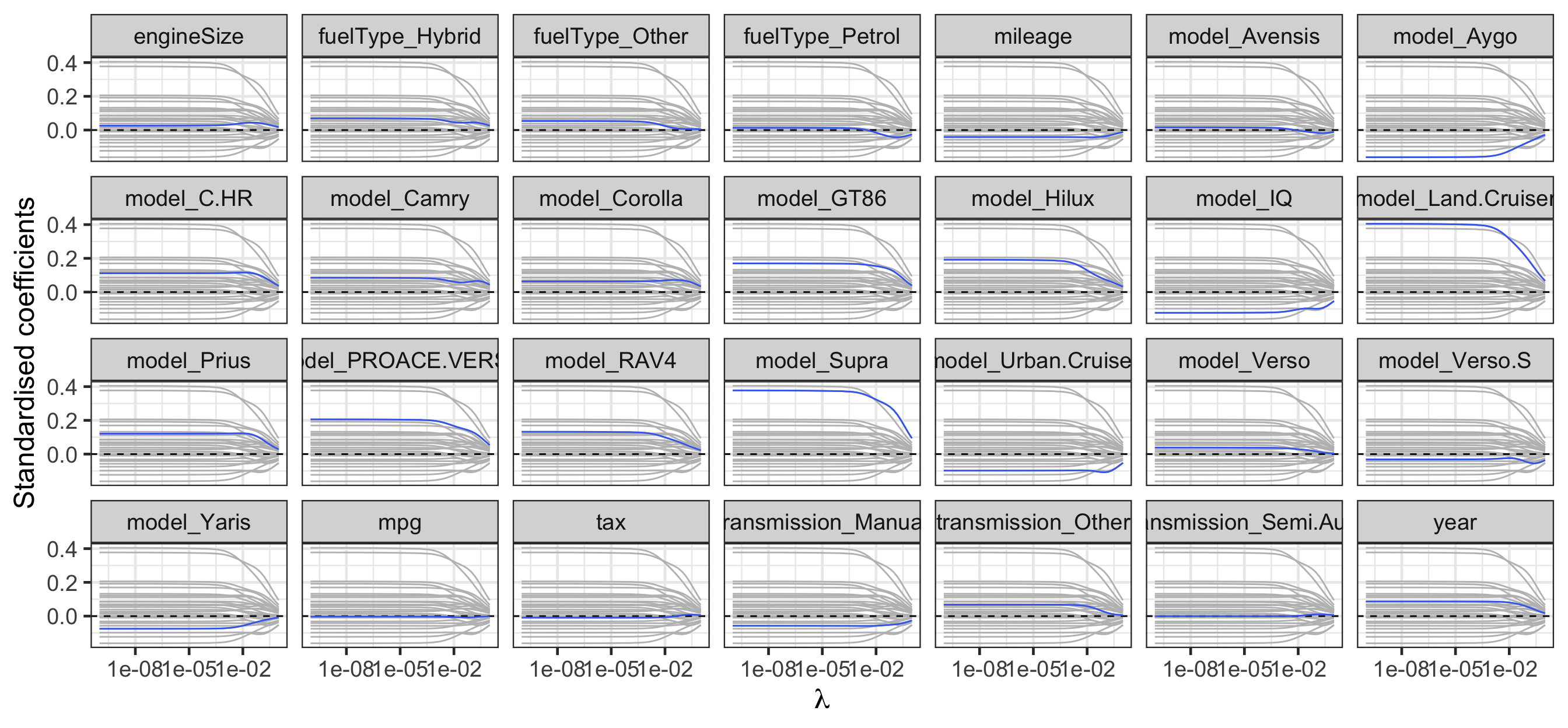
Selecting the tuning parameter \(\lambda\)
scroll
cv_glmnet_to_toyota <- function(alpha) {
  # Note: you're applying cross validation to the training dataset!
  toyota_train %>%
    # make the 10-fold cross validation data set
    vfold_cv(v = 10) %>%
    # for each fold, calculate the model metrics
    mutate(metrics = map(splits, function(.split) {
      # get the fold training dataset
      fold_train_data <- training(.split)

      # fit the model to the fold training dataset
      fold_fit <- glmnet(x = fold_train_data %>%
                                        select(-price),
                         y = fold_train_data$price,
                         alpha = alpha,
                         lambda = lambda_vec)

      # now get the validation dataset
      fold_test_data <- testing(.split)

      # get the predictions for this fold and models
      fold_preds <- fold_fit %>%
          predict(as.matrix(select(fold_test_data, -price))) %>%
          as.data.frame() %>%
          add_column(price = fold_test_data$price) %>%
          pivot_longer(-price, values_to = ".pred", names_to = "name") %>%
          left_join(tibble(name = paste0("s", 1:length(lambda_vec) - 1),
                           lambda = rev(lambda_vec)),
                    by = "name")

      # get the model metrics for this fold
      fold_preds %>%
          group_by(name, lambda) %>%
          metric_set(rmse, mae, mape)(., price, .pred) %>%
          select(-.estimator) %>%
          arrange(.metric, lambda)

  })) %>%
  # summarise the model metrics for each value of lambda
  unnest(metrics) %>%
  group_by(name, .metric) %>%
  summarise(lambda = unique(lambda),
            mean = mean(.estimate),
            se = sd(.estimate))
}
Tuning parameter for ridge regression
# A tibble: 150 × 5
# Groups:   name [50]
   name  .metric  lambda   mean      se
   <chr> <chr>     <dbl>  <dbl>   <dbl>
 1 s0    mae     1       0.104  0.00353
 2 s0    mape    1       2.59   0.0903
 3 s0    rmse    1       0.140  0.00490
 4 s1    mae     0.625   0.0891 0.00292
 5 s1    mape    0.625   2.22   0.0757
 6 s1    rmse    0.625   0.121  0.00451
 7 s10   mae     0.00910 0.0327 0.00130
 8 s10   mape    0.00910 0.817  0.0360
 9 s10   rmse    0.00910 0.0454 0.00366
10 s11   mae     0.00569 0.0325 0.00132
# … with 140 more rows
Selecting the tuning parameter for ridge regression
Code
toyota_tuning_ridge_min <- toyota_tuning_ridge %>%
               group_by(.metric) %>%
               filter(mean == min(mean))


toyota_tuning_ridge %>%
  ggplot(aes(lambda, mean)) +
  geom_errorbar(aes(ymin = mean - se,
                    ymax = mean + se)) +
  geom_line() +
  geom_point(data = toyota_tuning_ridge_min,
             color = 'red') +
  facet_wrap(~.metric, scales = "free") +
  scale_x_log10(name = latex2exp::TeX("\\lambda"))
| Metric | \(\lambda\) | Mean | Std. Error |
|---|---|---|---|
| rmse | 0.0001326 | 0.0445490 | 0.0039625 |
| mae | 0.0000000 | 0.0322999 | 0.0013496 |
| mape | 0.0000000 | 0.8054924 | 0.0367295 |
Fitting the ridge regression model
- Even though the context of this machine learning is linear regression, the interface for
glmnetis different tolmthat used a symbolic model formula. - Ideally these interfaces are standardised, but as methods are developed often by independent parties, differences often arise.
- It is important that you learn to make use of documentation and fit toy models to understand what functions are doing.
A tidy, unified interface with tidymodels 📦
parsnip(part oftidymodels) standardises this interface.
workflow(toyota_recipe) %>%
  add_model(linear_reg(engine = "glmnet", penalty = best_lambda_ridge, mixture = 0)) %>%
  fit(testing(toyota_splits)) %>%
  tidy()
# A tibble: 27 × 3
term estimate penalty
<chr> <dbl> <dbl>
1 (Intercept) 4.11 0.000133
2 year 0.0827 0.000133
3 mileage -0.0463 0.000133
4 tax -0.00728 0.000133
5 mpg -0.00608 0.000133
6 engineSize 0.0369 0.000133
7 model_Avensis -0.0310 0.000133
8 model_Aygo -0.129 0.000133
9 model_C.HR 0.115 0.000133
10 model_Camry 0.0283 0.000133
# … with 17 more rowsLimitation of ridge regression
- It will always use all \(p\) predictors!
- While it shrinks coefficients towards zero, it does not set it exactly to zero.
- Lasso is an alternative approach that induces a sparse model.
Lasso
Lasso
- Least absolute shrinkage and selection operator (lasso) is similar to ridge regression except for the constraint of the optimization problem:
\[{\hat{\boldsymbol\beta}_{lasso} = \underset{\boldsymbol\beta\in\mathbb{R}^{p+1}}{\mbox{arg min}}\ \text{RSS}(\boldsymbol{\beta})}\quad \color{#006DAE}{\text{subject to } \sum_{j=1}^p|\beta_j|\le s}.\]
Visualising the lasso constraint
- \(s\) bounds the magnitude of the coefficients.
- If \(s = 0\), all betas are equal to zero.
- If \(s = \infty\), then the LASSO = OLS.
- Axis grid:
X: \(\beta_1\)Y: \(\beta_2\)
Visualising the lasso
- For LASSO, \(\hat{\beta}_2 = 0\)!
- LASSO produces sparse models.
- Axis grid:
X: \(\beta_1\)Y: \(\beta_2\)Z: \(\text{RSS}(\beta_1, \beta_2)\)
Unconstrained representation for lasso
\[\hat{\boldsymbol\beta} = \underset{\boldsymbol\beta\in\mathbb{R}^{p+1}}{\mbox{arg min}}\left\{~\text{RSS}(\boldsymbol{\beta}) + \underbrace{\lambda \sum_{j=1}^p |\beta_j|}_{\large\text{shrinkage penalty}}\right\}\]
- \(\lambda \geq 0\) is a tuning parameter.
- Larger \(\lambda\) more shrinkage, smaller \(\lambda\) less shrinkage.
- \(\lambda\) can be chosen again via cross-validation.
Lasso in R
- Lasso for a particular \(\lambda\) can also be fit using the
glmnetpackage.
- Note here that the
alpha = 1(again, we’ll explain why later).
Regularisation path for lasso
Code
library(broom) # for tidy
est_lasso <- fit_lasso %>%
  tidy(return_zeros = TRUE)

est_lasso %>%
  filter(term != "(Intercept)") %>%
  mutate(zero = estimate == 0) %>%
  ggplot(aes(lambda, estimate))  +
  geom_line(data = ~rename(., term2 = term),
            aes(group = term2),
            color = "grey") +
  geom_hline(yintercept = 0, linetype = "dashed") +
  geom_line(aes(color = zero, group = term)) +
  facet_wrap(~term, nrow = 4) +
  labs(x = latex2exp::TeX("\\lambda"),
       y = "Standardised coefficients") +
  guides(color = "none") +
  scale_x_log10()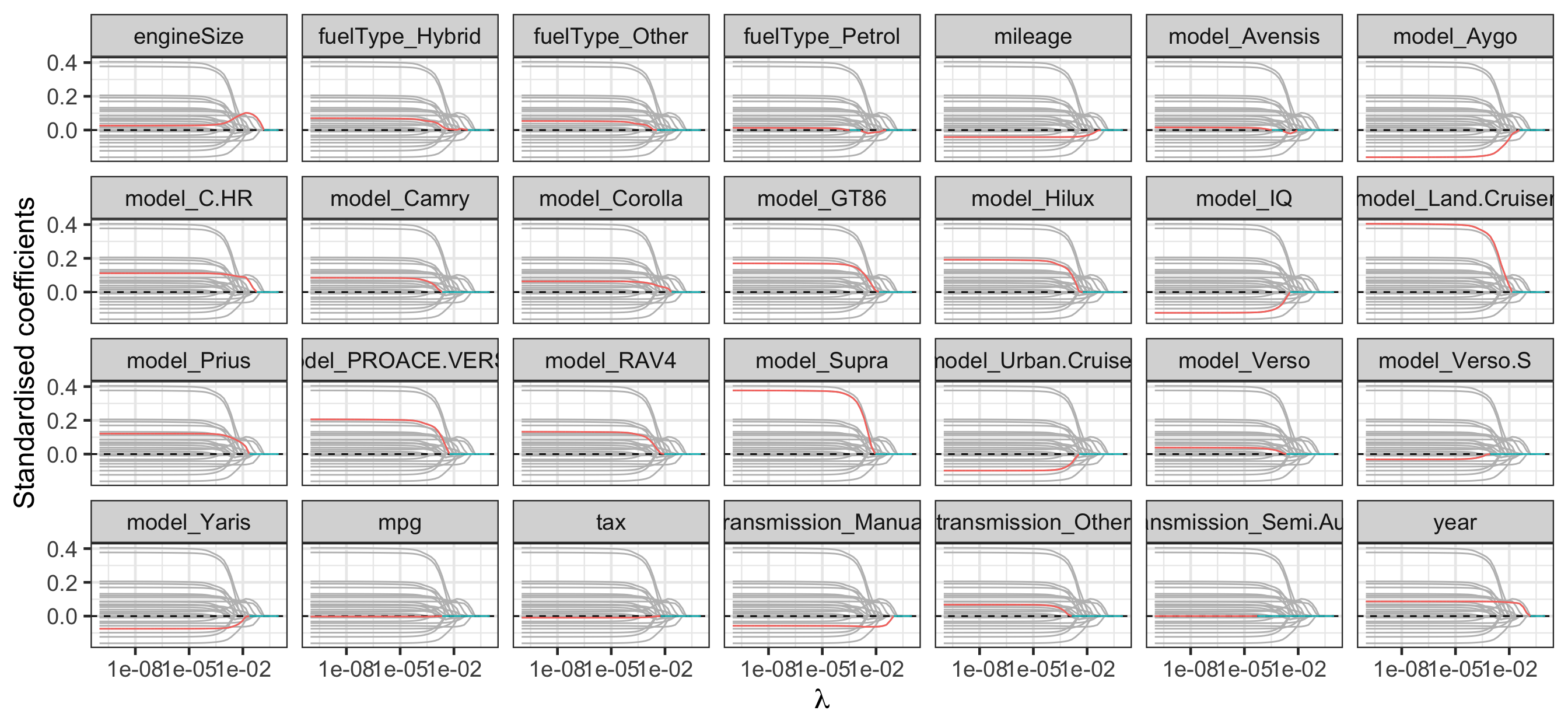
Selecting the tuning parameter \(\lambda\) for lasso
Code
toyota_tuning_lasso <- cv_glmnet_to_toyota(alpha = 1)

toyota_tuning_lasso_min <- toyota_tuning_lasso %>%
  group_by(.metric) %>%
  filter(mean == min(mean))

toyota_tuning_lasso %>%
  ggplot(aes(lambda, mean)) +
  geom_errorbar(aes(ymin = mean - se,
                    ymax = mean + se)) +
  geom_line() +
  geom_point(data = toyota_tuning_lasso_min,
             color = 'red') +
  facet_wrap(~.metric, scales = "free") +
scale_x_log10(name = latex2exp::TeX("\\lambda")) 
| Metric | \(\lambda\) | Mean | Std. Error |
|---|---|---|---|
| mae | 0 | 0.0323048 | 0.0017061 |
| mape | 0 | 0.8057043 | 0.0447169 |
| rmse | 0 | 0.0446230 | 0.0039084 |
Lasso limitations
- If a group of predictors are highly correlated, lasso will pick one of them at random, which is not desirable!
- There may be a grouping structure amongst the variables (e.g. dummy variables that belong to the same categorical variable) – in lasso, grouped variables are not simultaneously zero, which can result in only a subset of levels of a categorical variable being selected.
Group lasso
- We can change the penalty to induce a group sparsity.
\[\hat{\boldsymbol\beta}_{glasso} = \underset{\boldsymbol\beta\in\mathbb{R}^{p+1}}{\mbox{arg min}}\left\{~\text{RSS}(\boldsymbol{\beta}) + \lambda \sum_{j}||\boldsymbol{\beta}_j||\right\}\]
- \(\boldsymbol{\beta}_j\) denotes the vector of regression coefficients corresponding to the \(j\)-th group.
- \(\beta_{jk}\) denotes the \(k\)-th regression coefficient in the \(j\)-th group.
- \(||\boldsymbol{\beta}_j||\) denotes the Euclidean (\(L_2\)) norm of \(\boldsymbol{\beta}_j\).
Group lasso in R
- Group lasso for a particular \(\lambda\) can be fit using the
grpregpackage.
 [1] "year"         "mileage"      "tax"          "mpg"          "engineSize"
 [6] "model"        "model"        "model"        "model"        "model"
[11] "model"        "model"        "model"        "model"        "model"
[16] "model"        "model"        "model"        "model"        "model"
[21] "model"        "model"        "transmission" "transmission" "transmission"
[26] "fuelType" "fuelType" "fuelType" Regularisation path for group lasso
Code
est_glasso <- fit_glasso %>%
  broom:::tidy.glmnet(return_zeros = TRUE)

est_glasso %>%
  mutate(zero = estimate == 0) %>%
  filter(term != "(Intercept)") %>%
  ggplot(aes(lambda, estimate))  +
  geom_line(data = ~rename(., term2 = term),
            aes(group = term2),
            color = "grey") +
  geom_hline(yintercept = 0, linetype = "dashed") +
  geom_line(aes(color = zero, group = term)) +
  facet_wrap(~term, nrow = 4) +
  labs(x = latex2exp::TeX("\\lambda"),
       y = "Standardised coefficients") +
  scale_x_log10() +
  guides(color = "none")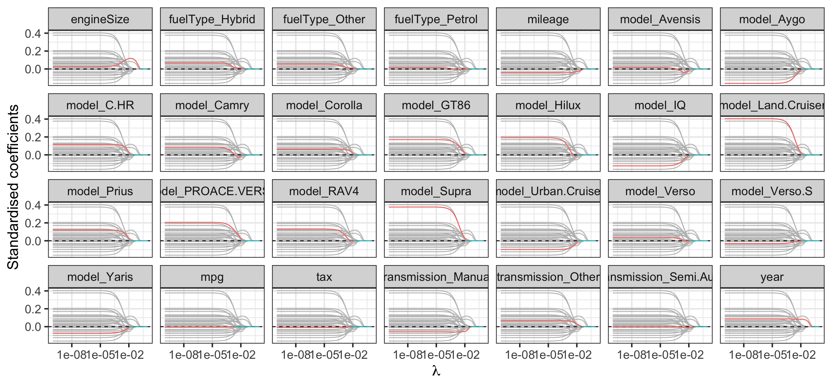
Regularisation path: lasso vs group lasso
scroll
Code
bind_rows(mutate(est_lasso, type = "lasso"),
          mutate(est_glasso, type = "glasso")) %>%
  mutate(type = fct_inorder(type),
         zero = estimate == 0) %>%
  filter(str_detect(term, "^(model_|transmission_)")) %>%
  ggplot(aes(lambda, estimate))  +
  geom_hline(yintercept = 0, linetype = "dashed") +
  geom_line(aes(group = interaction(term, type), color = type)) +
  facet_wrap(~term) +
  labs(x = latex2exp::TeX("\\lambda"),
       y = "Standardised coefficients") +
  scale_x_log10() +
  scale_color_manual("", values = c("royalblue2", "violetred2"))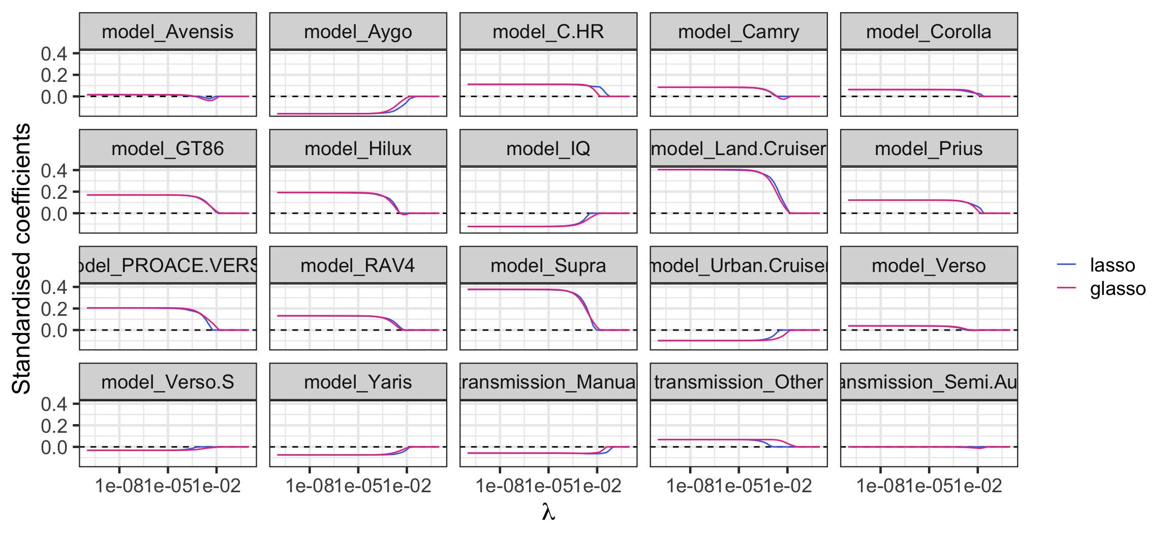
Visualising the constraints
Lasso
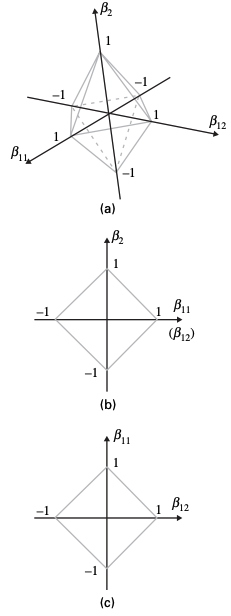
Group lasso
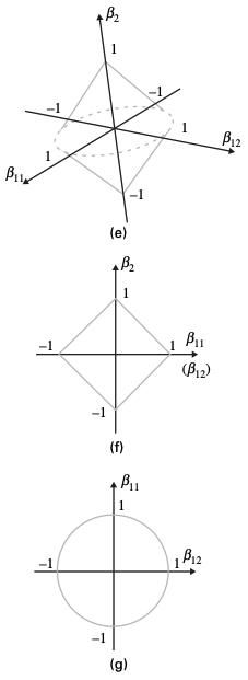
Ridge regression
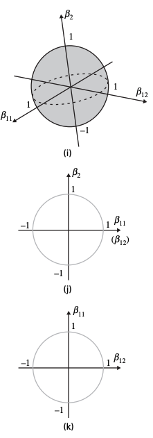
Elastic net
Elastic net
- Elastic net is an approach that combines LASSO and ridge regression.
\[\hat{\boldsymbol\beta}_{elastic} = \underset{\boldsymbol\beta\in\mathbb{R}^{p+1}}{\mbox{arg min}}\ \left\{\text{RSS}(\boldsymbol{\beta})+\lambda\left(\frac{1-\alpha}{2}\sum_{j=1}^p\beta_j^2+\alpha\sum_{j=1}^p|\beta_j|\right)\right\}.\]
- \(\alpha\) is another tuning parameter.
- If \(\alpha = 1\), elastic net = lasso.
- If \(\alpha = 0\), elastic net = ridge regression.
- You can pick \(\lambda\) and \(\alpha\) via cross-validation.
Takeaways
- Shrinkage methods are a powerful variable selection approach for regression by shrinking the coefficients predictors towards zero.
- You can use cross-validation to calibrate these methods for prediction.

ETC3250/5250 Week 3B