Code
This dataset is available from http://research.stlouisfed.org/fred2.
\color{#006DAE}{y_i = \beta_0 + \beta_1x_{i1}+ \beta_2x_{i1}^2 + \cdots + \beta_{27}x_{i1}^{27} + e_i}
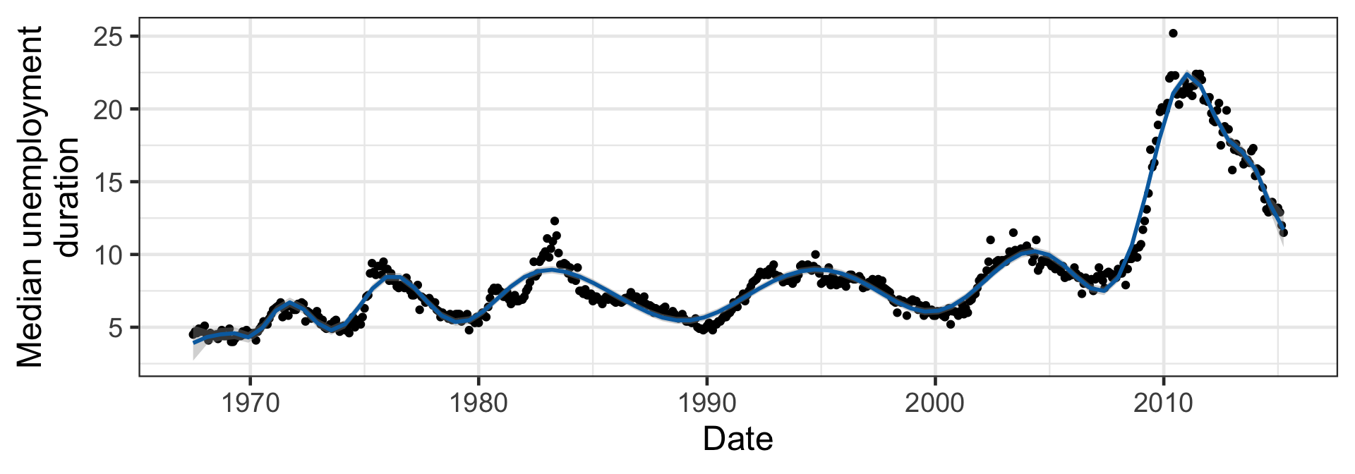
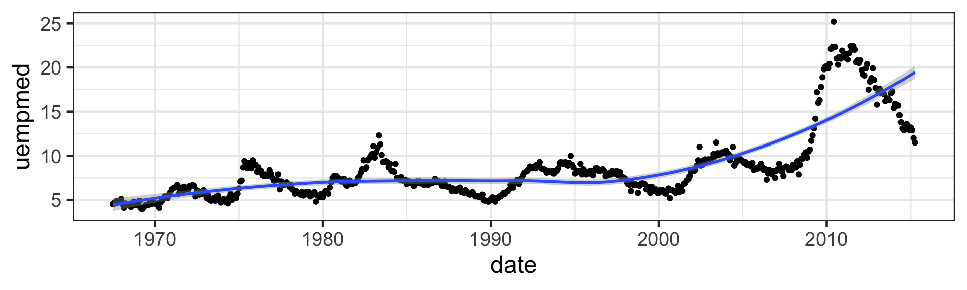
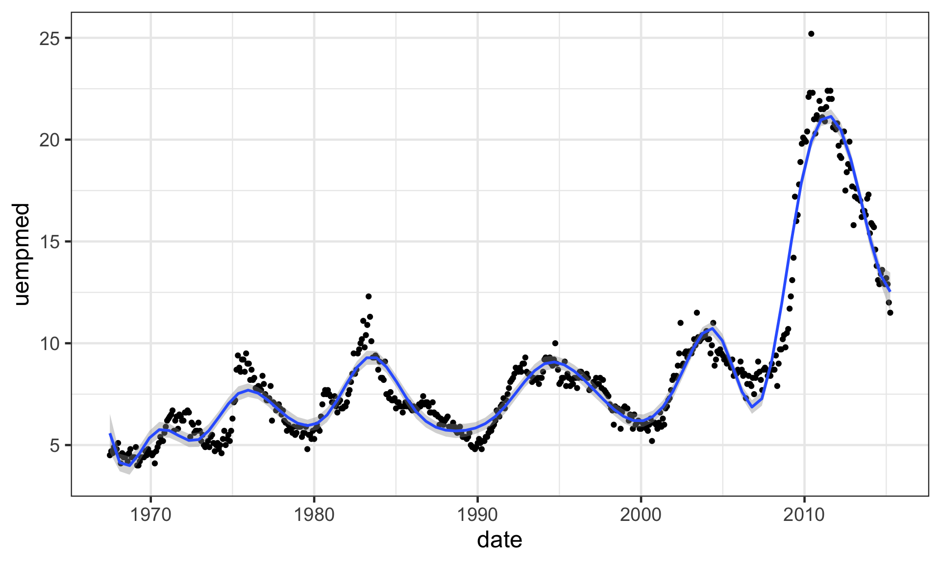
In ggplot, you can add the loess using geom_smooth with method = loess and method arguments passed as list:
span changes the loess fit
loess works
.png)
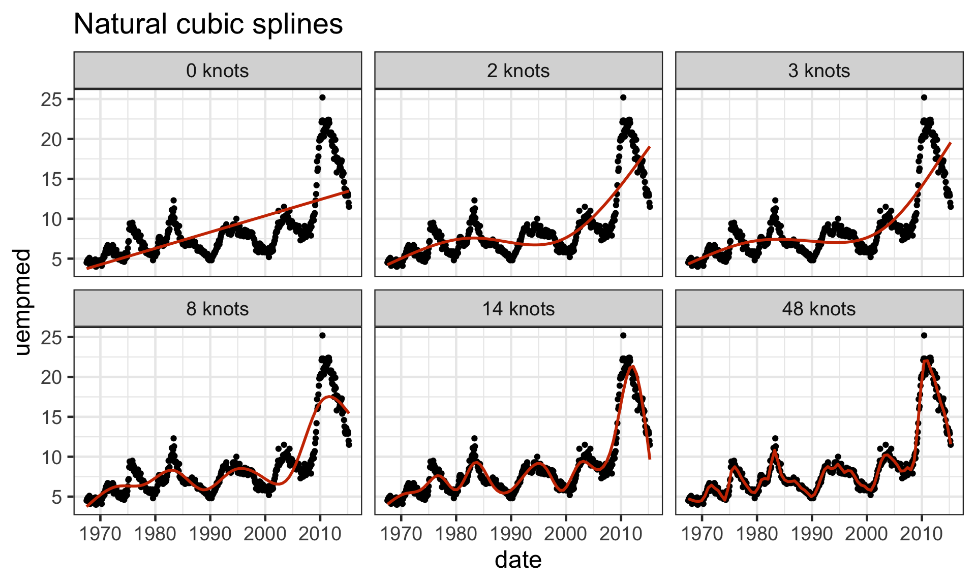
map_dfr(c(0, 2, 3, 8, 14, 48),
        ~ economics %>%
          mutate(
            nknot = .x,
            nknot_label = paste(nknot, "knots") %>% fct_inorder()
          )) %>%
  ggplot(aes(date, uempmed, nknot = nknot)) +
  geom_point() +
  geom_smooth(
    method = lm,
    formula = y ~ splines::ns(x, df = nknot + 1),
    se = FALSE,
    colour = "orangered3"
  ) +
  facet_wrap(~ nknot_label) +
  ggtitle("Natural cubic splines")