Toyota dealer
- You need to price a second-hand 2004 Toyota Yaris for a car dealer.
.jpg)
_Ascent_sedan_(2018-08-27)_01.jpg)
_–_Frontansicht,_21._Juli_2012,_Heiligenhaus_(cropped).jpg)
- You make use of this Toyota used car listing data.
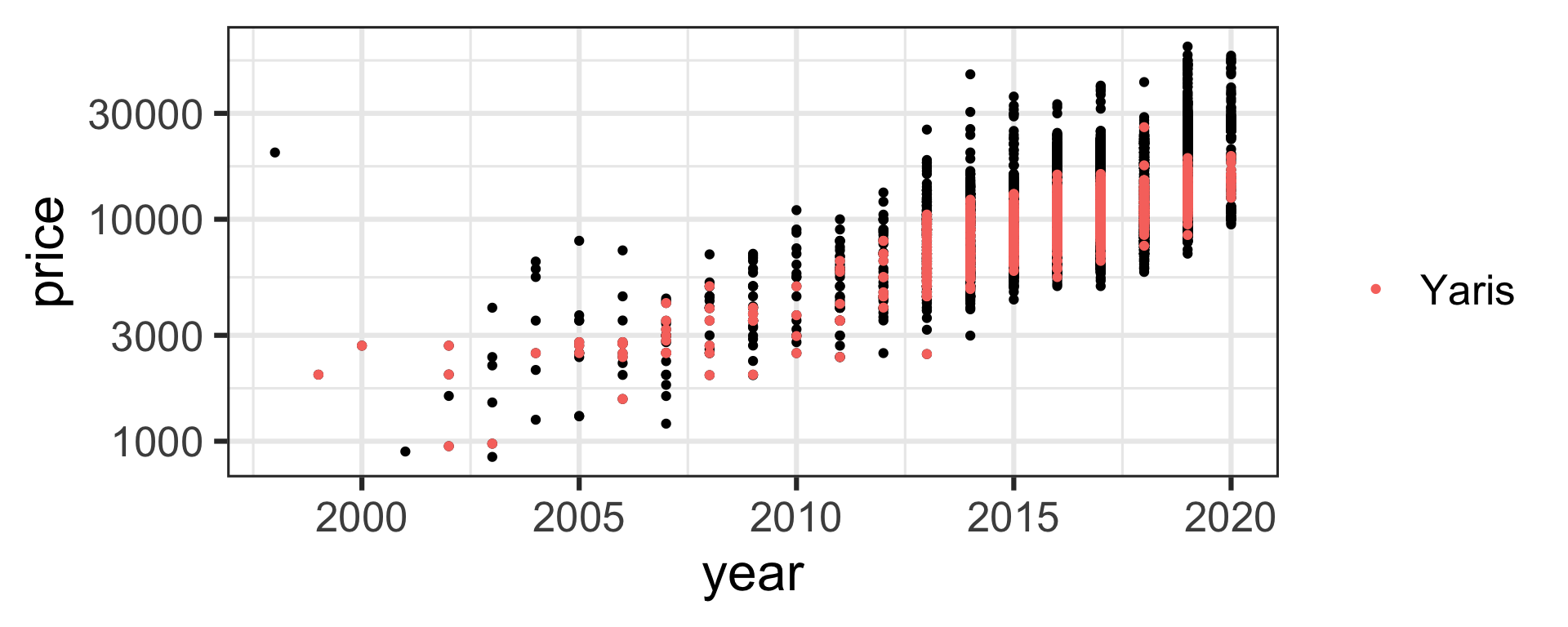
Car price as a function of year
- Let’s consider the (log of) Toyota Yaris car price as a function of year.
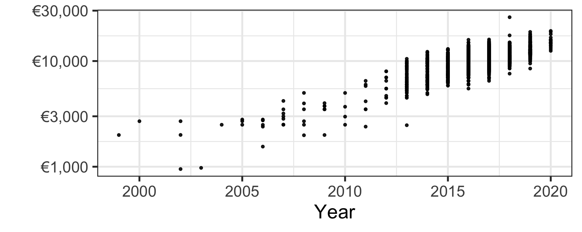
- The car price is generally higher for cars made more recently.
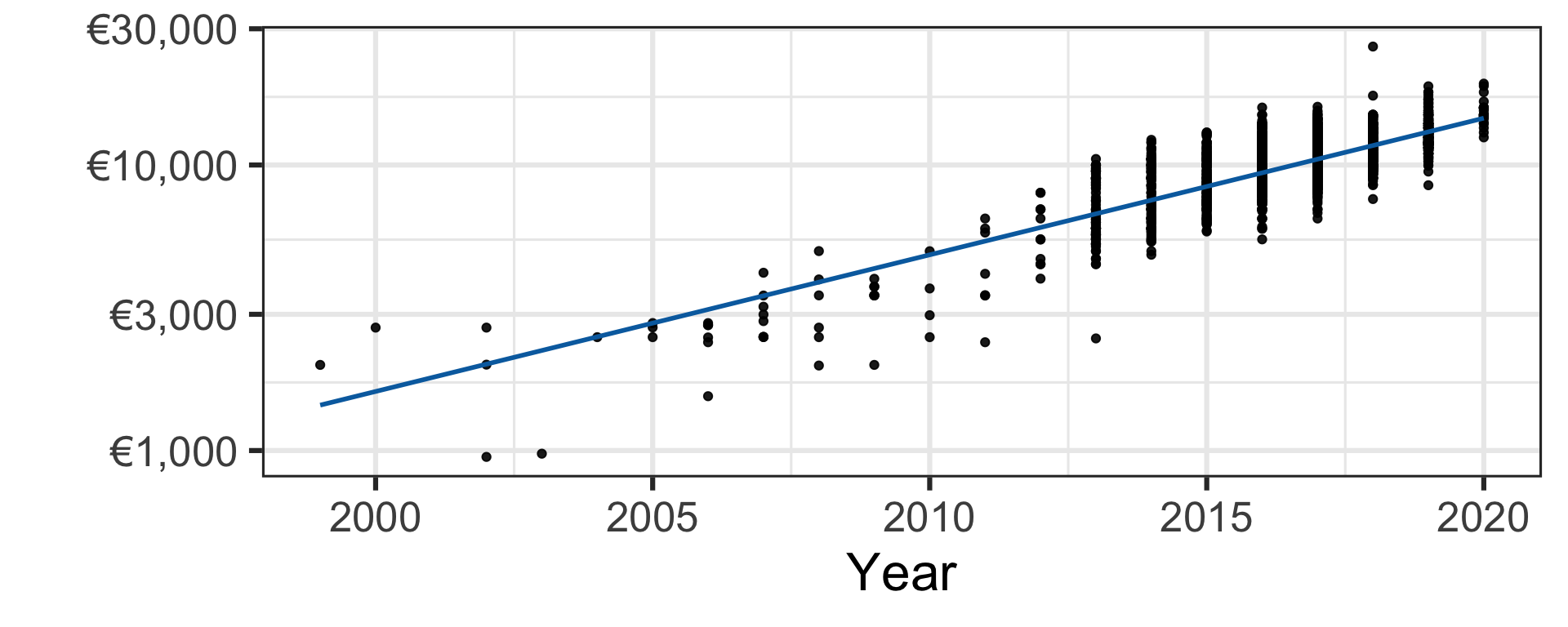
Simple linear regression
- Let’s fit the line of best fit using the least squares approach.
Simple linear regression
- Let’s fit the line of best fit using the least squares approach.
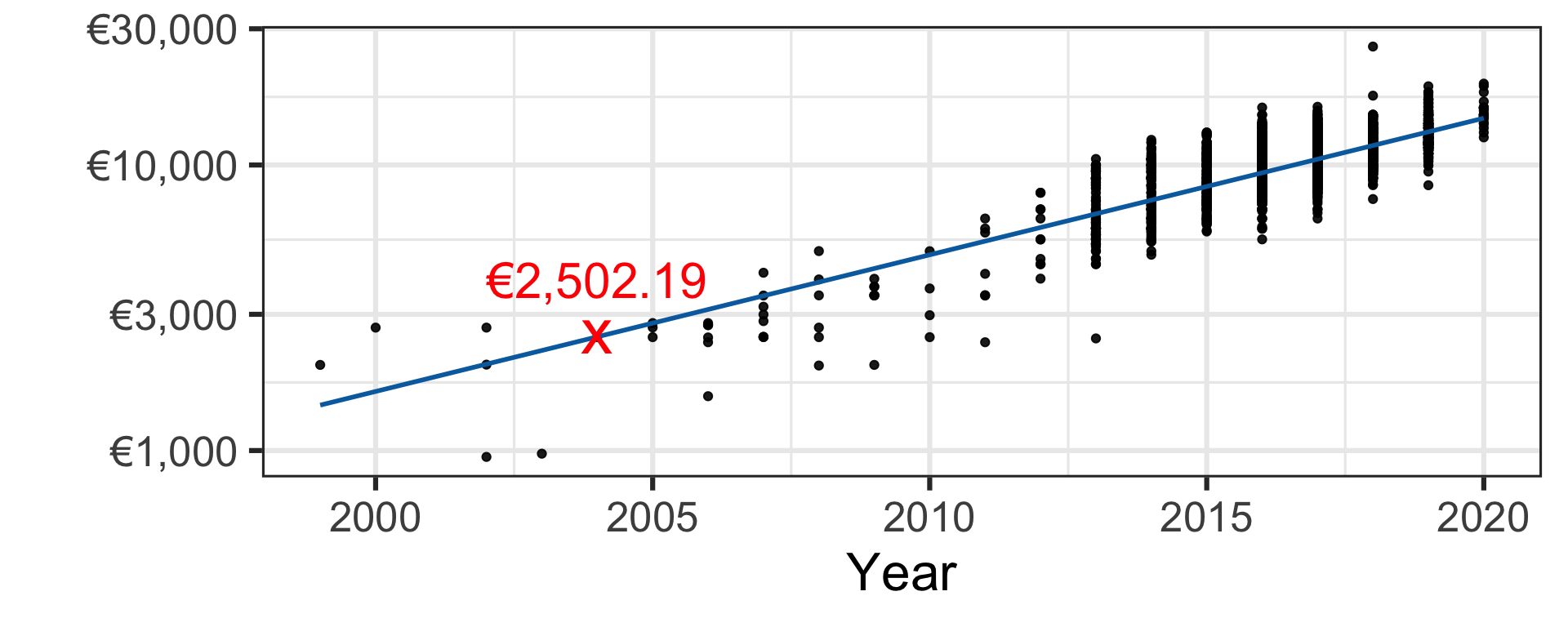
- Under this (simplistic) model, we would price a second-hand 2004 Toyota Yaris as €2,502.19.
Simple linear regression
Pricing a second-hand 2004 Toyota Yaris car
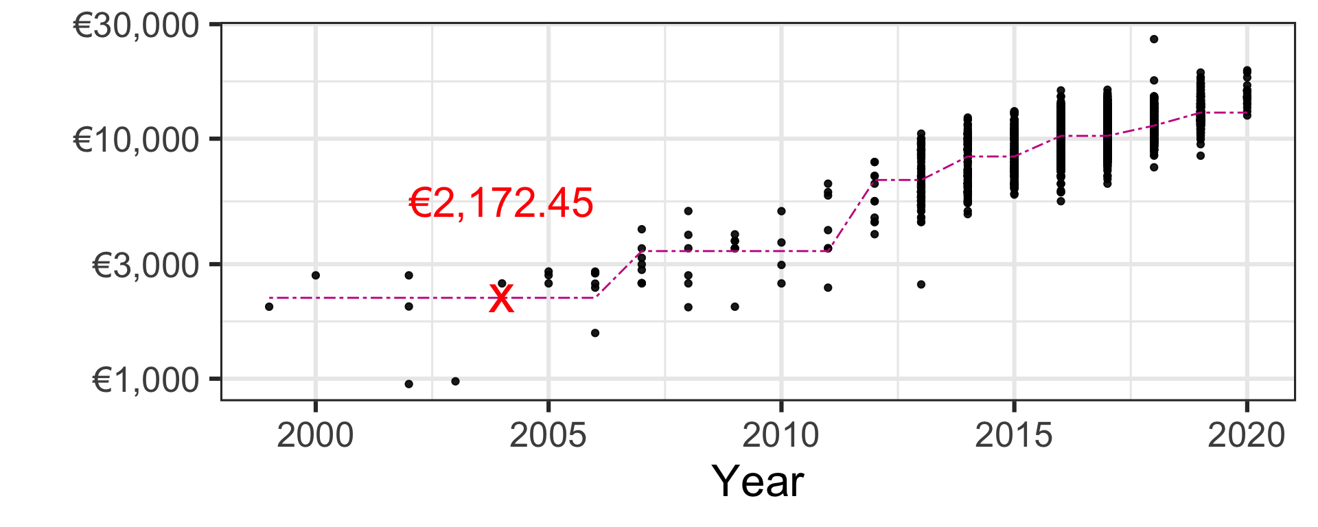
Regression trees
Pricing a second-hand 2004 Toyota Yaris car
For now don’t worry how this is calculated - we will learn this later.
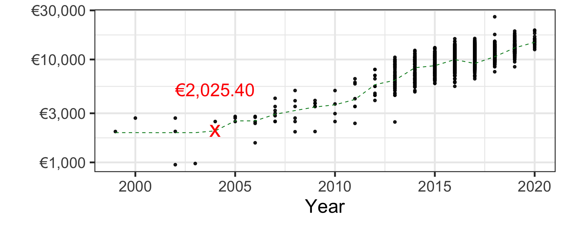
k-nearest neighbour
Pricing a second-hand 2004 Toyota Yaris car
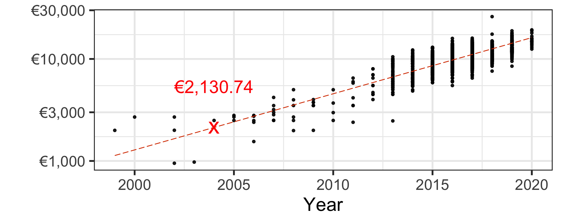
Neural network
Pricing a second-hand 2004 Toyota Yaris car
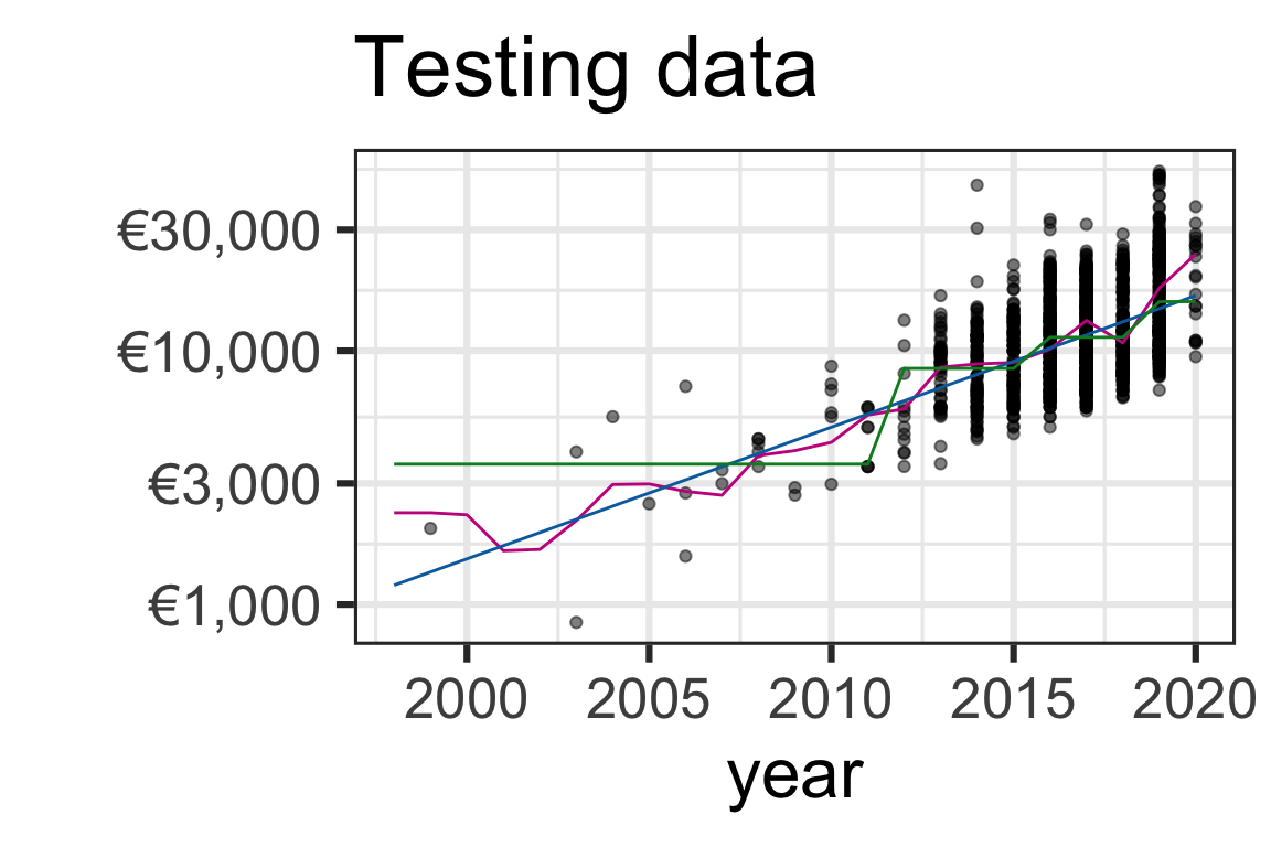
Comparing models for regression problem
Pricing a second-hand 2004 Toyota Yaris car
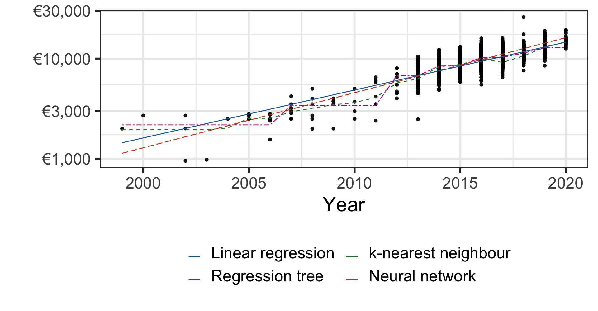
| Method | Price |
|---|---|
| Linear regression | €2,502.19 |
| Regression tree | €2,172.45 |
| k-nearest neighbour | €2,025.40 |
| Neural network | €2,130.74 |
- Which model to use? How to choose parameters?
We’ll come back to these questions later.
Breast cancer diagnosis

Image from American Cancer Society website

Image from Street et al. (1993) Nuclear feature extraction for breast tumor diagnosis. Biomedical Image Processing and Biomedical Visualization 1905 https://doi.org/10.1117/12.148698
- We use the Wisconsin breast cancer data set to build a model to predict if the breast mass sample is malignant (M) or benign (B).
- Here the response is categorical with two classes (M and B).
Features from the digitized image from FNA
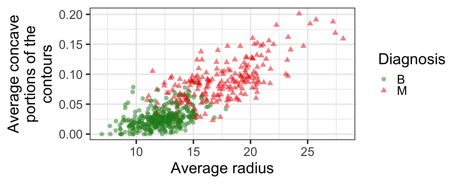
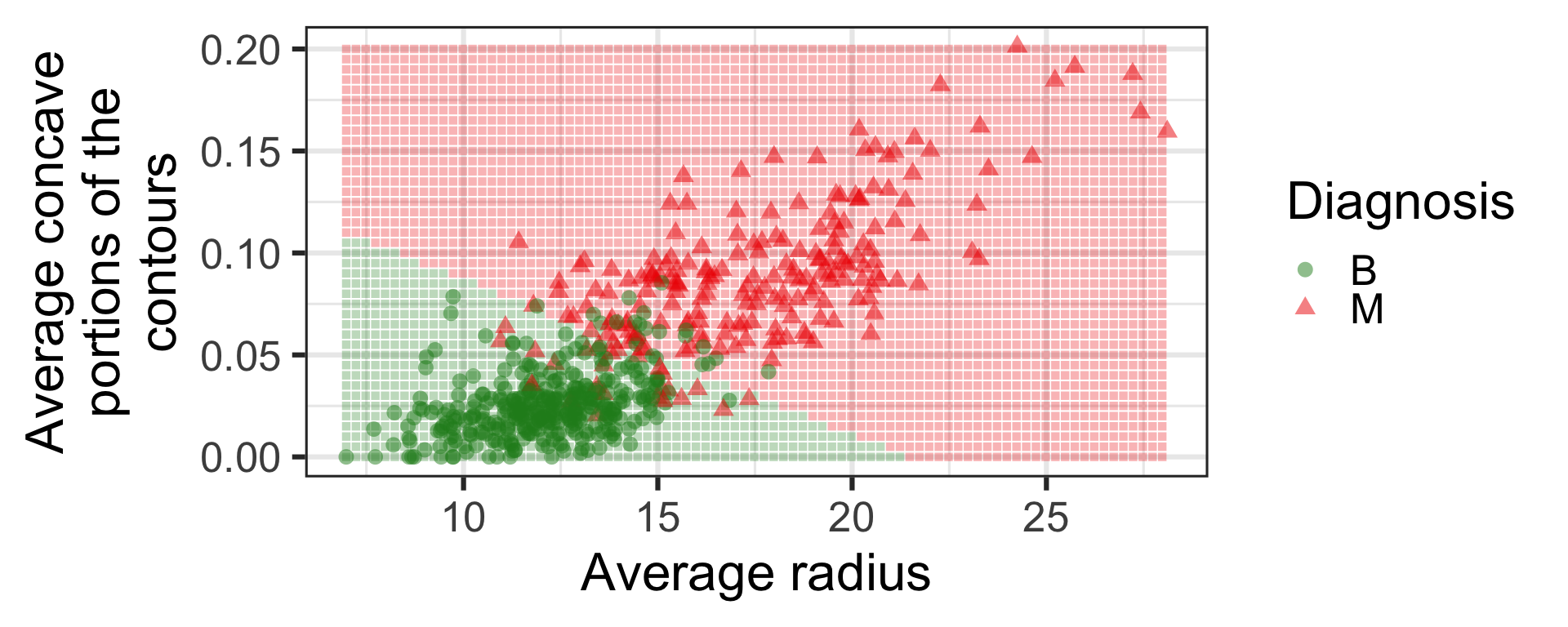
- Before fitting any model, we can already see that the average radius and concave portions in the digitized image separate out the two classes.
Logistic regression
Again don’t worry how this is calculated - we will cover this in Week 4.
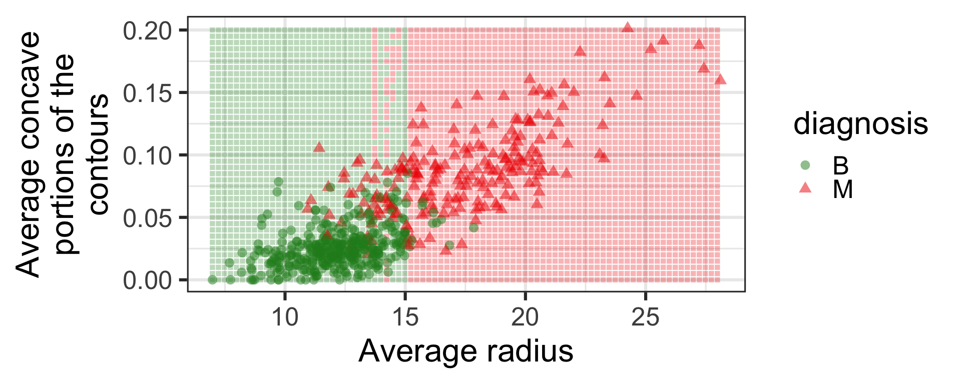
k-nearest neighbour
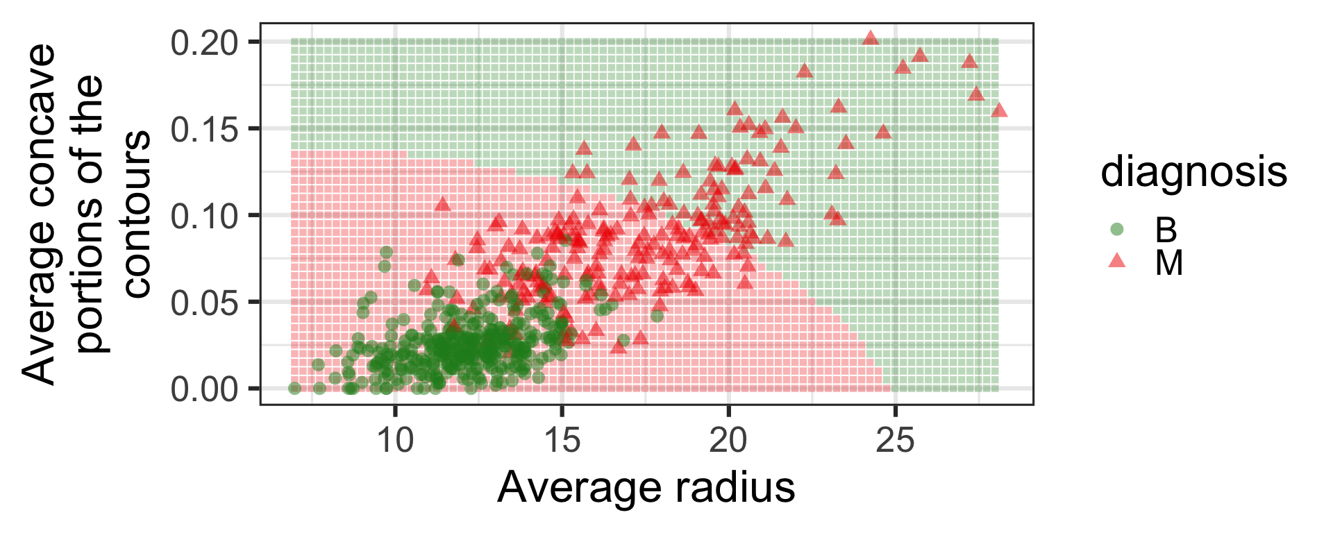
Neural network
- What would you do to choose which model to use?
We’ll talk more on this later.
Dimension reduction and clustering
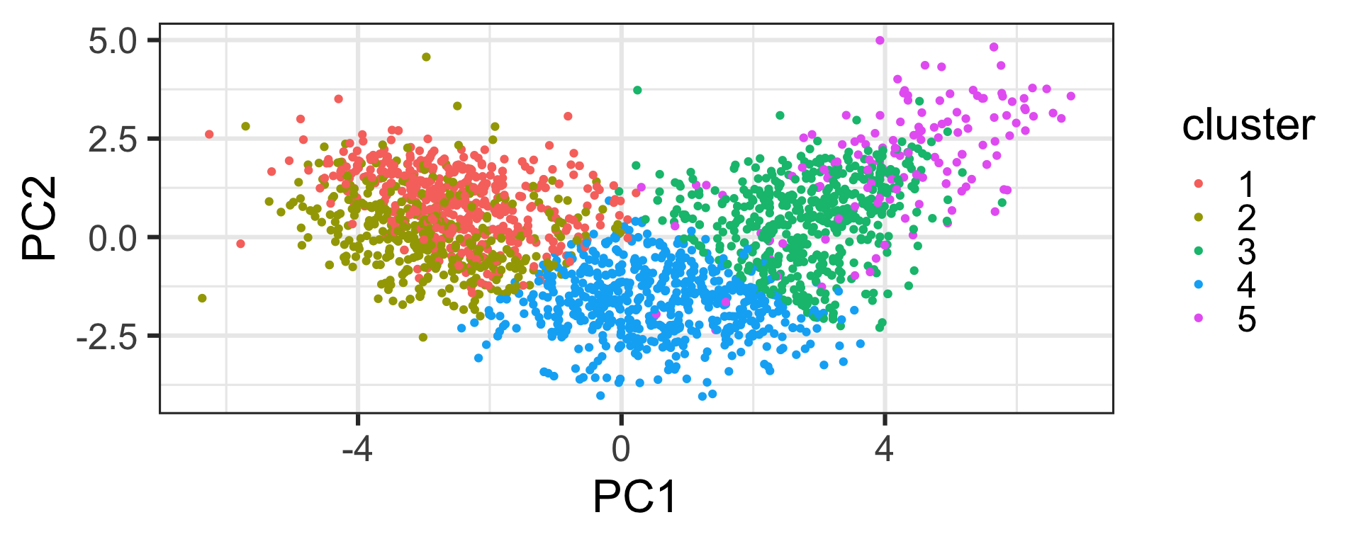
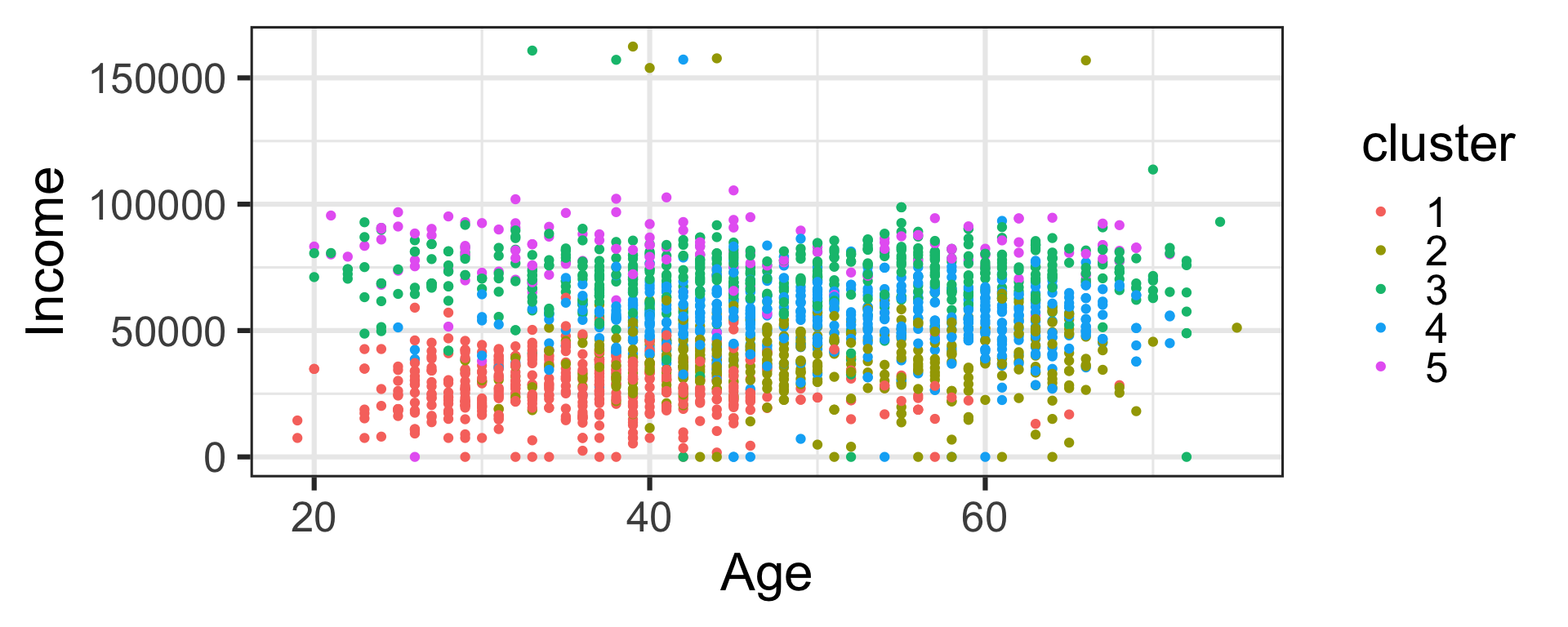
- Data with too many variables is hard to understand or process.
- We can reduce dimension in a meaningful way.
- Or cluster similar groups together to find inherent grouping structure.
Training, validation and testing data sets
- In machine learning, three data sets are commonly used to build and select the model:
- training data is used to fit the initial model
- validation data is used to evaluate the model fit from the training data to help tune the hyperparameters
- testing data (or holdout data) is used to evaluate the tuned model
- We’ll denote the set of index of training data, validation data and testing data as Train, Valid and Test, respectively.

Image from Emi’s blog
A linear regression
- A proposed model is \log_{10}(\texttt{price}_i) = \beta_0 + \beta_1 \texttt{year}_i + e_i
Visualising the predictions
Code
results_pred <- imap_dfr(model_fits, ~{
    tibble(year = seq(min(toyota$year), max(toyota$year))) %>%
      mutate(.pred = 10^predict(.x, .),
             .model = .y)
  })

gres <- ggplot(toyota_train, aes(year, price)) +
  geom_point(alpha = 0.5) +
  geom_line(data = results_pred, aes(y = .pred, color = .model)) +
  scale_color_manual(values = c("#C8008F", "#006DAE", "#008A25")) +
  scale_y_log10(label = scales::dollar_format(prefix = "€", accuracy = 1)) +
  theme(legend.position = "bottom") +
  labs(title = "Training data", y = "", color = "")  +
  guides(color = "none")


gres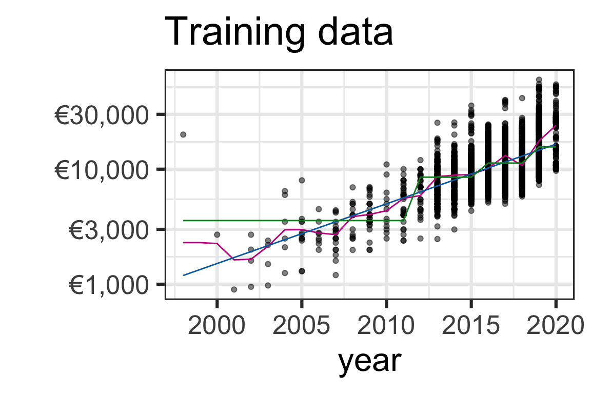
Select a model
- Based on the predictive accuracy, we may choose to select the regression tree for prediction (it has the best metric for all, except for MPE).
- But for inference, simple linear regression model has an easier interpretability.
- Selecting a model isn’t just about selecting the model with the best metric - data and problem context matters.

Takeaways
- There are diverse sets of problems where appropriate data with adequate machine learning is helpful in solving it.
- In order to compare predictive performance of machine learning models, we apply the trained models to the testing data.
- There are many methods to machine learning and various metrics to compare models – what is appropriate depends on the data, context and aim.
- To understand these methods and metrics, we will use some mathematics, go through variety of data and apply the models using R.