
devtools::install_version("edibble", version = "1.1.0", repos = "http://cran.rstudio.org")
Note
- The PDF version of this paper can be found on arxiv: https://arxiv.org/abs/2311.09705
- The paper uses edibble R package version 1.1.0 which can be installed as:
1 Introduction
The critical role of data collection is well captured in the expression “garbage in, garbage out” – in other words, if the collected data is rubbish, then no analysis, however complex it may be, can make something out of it. Experiments offer the highest degree of control in the method of data collection and are of a critical importance for validating or investigating hypotheses across numerous fields (e.g., agriculture, biology, chemistry, business, marketing, engineering). A proper design of experiments is critical to ensure that the desired inference is valid and efficient based on the experimental data. Conducting experiments is usually expensive; thus improper designs are at best inefficient use of resources and, at worst, a complete waste of resources. Given such high stakes, it is clear that improving the practice of experimental design can translate to large gains by increasing the inherent value of the experimental data.
However, more holistically, experiments involve multiple steps that extend beyond generating an experimental design table or layout. An appropriate experimental design cannot be generated without context and subject matter expertise to identify the appropriate experimental factors (Hahn 1984; Steinberg and Hunter 1984). Furthermore, the experimental design is useless if it is not carried out as intended or if there are issues with data entry. Generating an experimental design should not be seen as an isolated activity, but rather viewed as an interconnected activity within the life of the whole experiment. Even a fit-for-purpose analysis of experimental data is not an independent activity void of the knowledge of the experimental design. Naturally, we can develop systems for constructing experimental designs that support an integrated approach for the entire lifecycle of an experiment.
Many experimental design software programs do not offer an integrated approach. Rather, the software tightly integrates the algorithmic aspect into a given experimental structure, thus losing the flexibility to specify other structures (Tanaka and Amaliah 2022). Unfortunately, this tight integration causes friction when considering alternative algorithms and requires users to rebuild the specification from scratch for another software solution. In addition, because the processes to specify the design are generally not modular, users must process all aspects of the experimental design simultaneously, burdening their cognitive load. As an alternative framework to specify experimental designs, Tanaka (2023) presented a computational framework, called “the grammar of experimental designs”, which allows for intermediate constructs of experimental designs. This framework adopts a process-based approach to support the gathering of required information for the entire experiment in a modular manner.
In Tanaka (2023), an experimental design is treated as a mutable object that progressively builds to the final design by a series of functions that modify a targetted element of the experimental design. This system is applicable to a broad range of experimental designs with fixed levels for each experimental factor. The system can be understood as an analogy to grammar in linguistics; a vast array of experimental designs (sentences) is expressed by combining key functions (words) through the shared understanding of the rules (grammar). In this system, an intermediate construct of an experimental design is represented as a pair of directed acyclic graphs (DAGs), where the nodes of one DAG represent the experimental factors, whereas the nodes of the other DAG represent the levels of those factors. Users explicitly define the experimental factors, their roles (such as treatment, unit or record), and relationships between the nodes. These purposeful manipulations of the DAGs are invoked by a small collection of object methods. The names of these methods (e.g., “set units” and “assign treatments”) are semantically aligned to raise conscious awareness of the user (and the reader) to the elements of the experimental design. The edibble package in the R language (R Core Team 2023) was used to demonstrate the utility of the framework in Tanaka (2023), however, little explanation was given to the usage of the package.
This paper extensively demonstrates the main features of the edibble package. Section 2 provides an overview of its usage, Section 3 describes various methods for defining the experimental structure. Section 4 presents additional examples based on real experiments. Section 5 contrasts the existing systems. Finally, we conclude the paper with a discussion in Section 6.
2 Usage overview
The edibble package is available on the Comprehensive R Archive Network (https://cran.r-project.org/) with the latest developments available on GitHub at https://github.com/emitanaka/edibble. The code presented in this paper is based on version 1.1.0 of the edibble package.
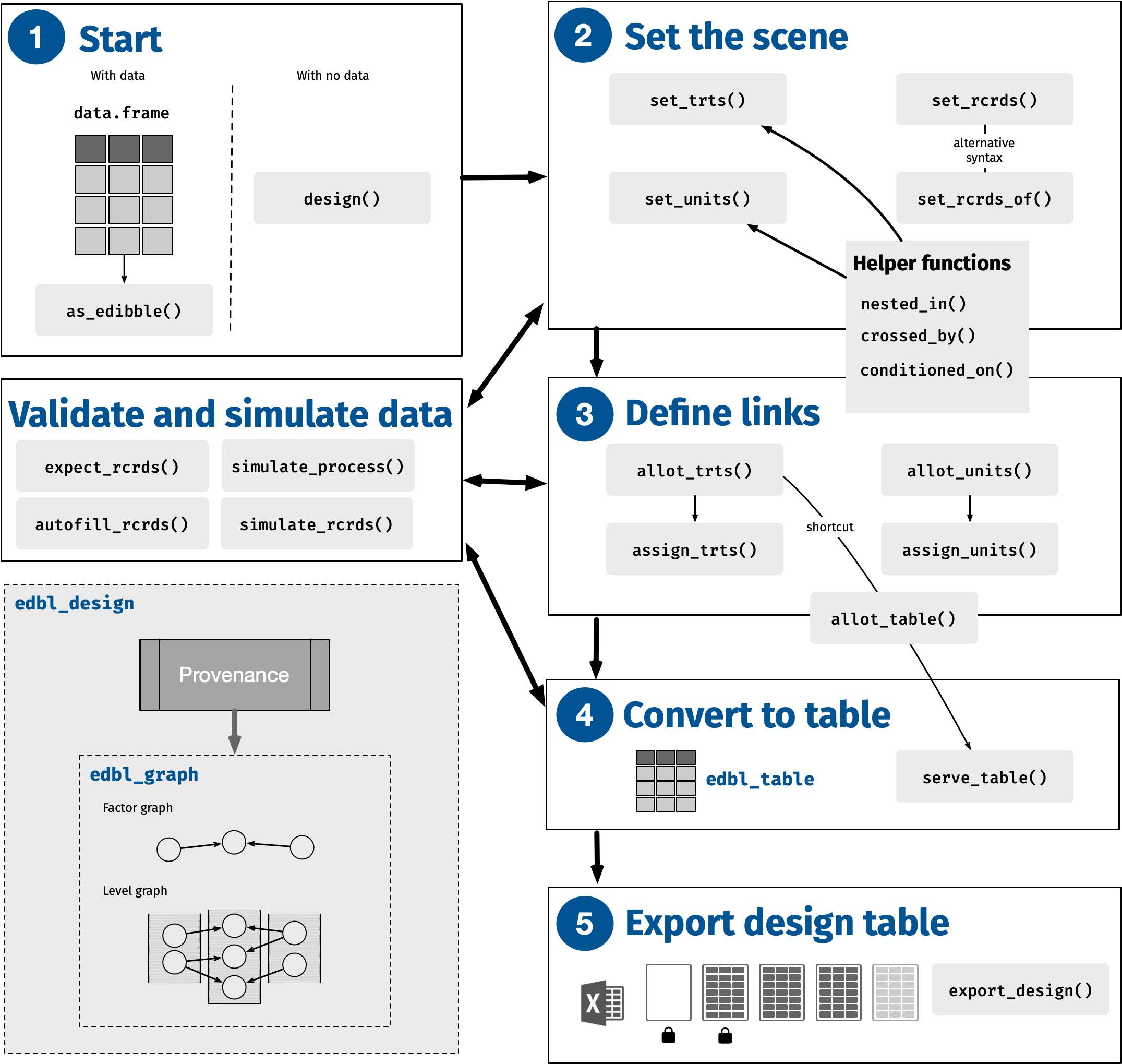
The ultimate aim of the edibble package is to produce an experimental design table. The name reflects this aim, with edibble standing for experimental design tibble, where tibble is a special type of data.frame from tibble package (Müller and Wickham 2023b). The key functions to achieve this aim are illustrated in Figure 1. An example shown next demonstrates a quick overview of its usage.
Consider Example 1, derived from the example in Bailey (2008) for a quick demonstration of the edibble package. The main aim of this experiment is to determine the best feed type for calves to gain weight.
Example 1: Calf feeding
There were 8 pens, with 10 calves in each pen. The experimenter was interested in comparing the effects of the four types of feed on the calves’ weights. Each calf was individually weighed. The four feeds were combinations of two types of hay, which were put into the pen, and two types of anti-scour treatments, which were administered individually to each calf.
To specify this experiment in edibble, we composed it using a series of functions as shown below. The pipe (%>%) function, imported from magrittr (Bache and Wickham 2022), allows for a series of nested operations and can be substituted with the native pipe (|>) available from R version 4.1.0 onwards. This style of coding would be familiar to users of tidyverse (Wickham et al. 2019).
library(edibble)
1calf <- design("Calf feeding") %>%
2  set_units(pen = 8,
            calf = nested_in(pen, 10)) %>%
3  set_rcrds(weight = calf) %>%
4  # set_trts(feed = 4) %>%
5  set_trts(hay = 2,
           antiscour = 2) %>%
6  allot_table(hay ~ pen,
antiscour ~ calf)- 1
- We begin the design specification by initiating the edbl_design object using design. An optional title is provided, which is encoded and persistently displayed at various outputs (e.g., print or export of the object).
- 2
- As described in the example, we had 8 pens with 10 calves in each pen. This part of the code specifies the unit factors “pen” and “calf”. The right hand side shows the number of levels as a single numerical value. The function nested_in is a helper function that encodes the calf is nested in pen.
- 3
-
As each calf is individually weighed, we set the records such that the weight is recorded for each calf (
weight = calf). Here, the right hand side has to be a unit factor that has been previously defined. - 4
-
We are told that we are comparing four types of feed; hence, we set the treatments to
feed = 4, but we realise later that this is not the entire description. We comment this line out and instead write our understanding in the next lines. You can, of course, choose to delete this line, but it can be useful to keep a record of your process.
- 5
- Here, we write our new understanding that the feed is composed of two types of hay and two types of anti-scour treatments.
- 6
- In the final step, allot_table is a short hand for allot_trts, assign_trts, and serve_table; as such, multiple processes occur in this call. The relationship between the units and treatments is specified: hay type is alloted and assigned randomly to the pen, and anti-scour treatment type is alloted and assigned randomly to the calf within the pen. The design object is then translated into a table.
Printing the object above shows the table below, in which each experimental factor is translated into a column.
calf# Calf feeding
# An edibble: 80 x 5
pen calf weight hay antiscour
<U(8)> <U(80)> <R(80)> <T(2)> <T(2)>
<chr> <chr> <dbl> <chr> <chr>
1 pen1 calf01 o hay2 antiscour2
2 pen1 calf02 o hay2 antiscour1
3 pen1 calf03 o hay2 antiscour2
4 pen1 calf04 o hay2 antiscour1
5 pen1 calf05 o hay2 antiscour1
6 pen1 calf06 o hay2 antiscour2
# ℹ 74 more rowsThe resultant object also contains the edbl_design object (hereafter referred plainly as the design object). The user may also plot the internal graphs using the plot function. By default, this shows the factor graph as an interactive plot by internally using the visNetwork package (Almende B.V. and Contributors and Thieurmel 2022). The level graph can be seen by adding the argument as which = "levels" in the plot function. The static plots of the factor and level graphs are shown in Figure 2. The level graph can contain many nodes since every level of each experimental factor, except the record factors, is shown.
plot(calf) # factor graph is default
plot(calf, which = "levels") # level graph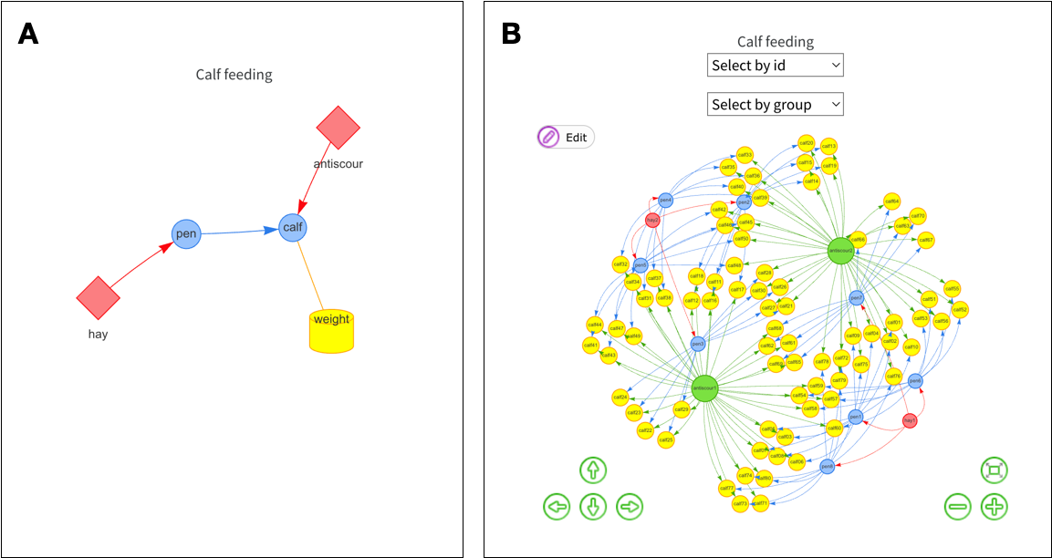
In experiments, there would be a response of interest. A response is often not required to generate an experimental layout. It is generally assumed that the smallest unit in the experimental design table is the observational unit (although not always so). In edibble, users can optionally specify their intention of what to record (e.g., responses) on which particular unit factor, as was done above, where the intention to capture the weight of each calf is specified in the function set_rcrds. We can further add the expectations of the values for the weight factor. For example, below, we use expect_rcrds to encode a data validation that the weight should be a numeric value between 0 and 10.
calfr <- calf %>%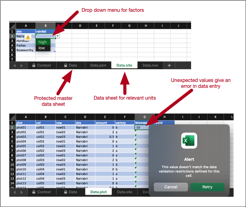
expect_rcrds(weight > 0, weight < 10)The benefit of encoding the data validation rule is that it is now interoperable. Two functionalities in edibble take advantage of this encoding. The first is when exporting the design through export_design. This outputs an Excel file with the column “weight” in the data sheet for calves. The cells in this column are empty, with the intention that the data collector enters the data in this Excel sheet. These cells have the data validation embedded such that if the entry is not a numeric value between 0 and 10, it will result in an error in the data entry. See more details in Section 3.5.1.
The other functionality in edibble that takes advantage of the data validation encoding is when simulating data for record factor(s). There are two approaches to simulating data in edibble: one that requires users to extensively describe the simulation process (simulate_process and then simulate_rcrds, and the other that automatically writes the simulation scheme for you while ensuring to generate valid values: autofill_rcrds. When users describe the simulation data on their own, it is possible to violate the valid values. In this case, the values are censored (by default to missing values) in simulate_rcrds. More details on the simulation capabilities are presented in Section 3.5.2.
3 Defining structure
An experimental structure always consists of a unit structure; in other words, an experiment cannot be defined without units. If the experiment is comparative, then it must consist of a treatment structure in addition to the mapping between the unit and treatment factors. This mapping can be defined on two levels: a high-level mapping between factors (usually for humans to understand the broad picture), and a low-level mapping between factor levels (usually assigned algorithmically).
There are three roles for the experimental factors that can be encoded in edibble: treatment, unit, and record (see more details in Tanaka 2023). The functions, set_trts, set_units, and set_rcrds are used to encode the treatment, unit, and record factors, respectively, into the design object. The calls to these functions are generally associative, that is, the order does not matter nor does the number of calls to it matter (e.g., you do not need to define all units in one call and instead call on set_units repeatedly). The exception is when the new factor is dependent on a previously defined factor; in this case, the dependent factor must be defined later.
Once the factors are defined, the relationship between them and their levels must be defined. The high-level grammar restricts the users in the type of relationships that can be defined (e.g., you cannot assign treatments to record factors), although low-level tweaks to the grammar (meant for developers) can bypass these restrictions (not presented in this paper).
The main functions in edibble are explained in detail In the following subsections. In this section, we assume that the experimental aim is to find the best wheat variety from a wheat field trial.
3.1 Initialisation
library(edibble)A new design constructed using edibble must start by initialising the design object. An optional title of the design may be provided as input. This information persists as metadata in the object and is displayed in various places (e.g., print output and exported files).
3.1.1 With data
If you have existing data, you can use it as a base to build the design object. Below, we convert the data gilmour.serpentine in agridat (Wright 2022) into an edbl_table object.
as_edibble(agridat::gilmour.serpentine,
           .title = "Wheat Experiment",
           .units = c(col, row, rep), .trts = gen)
# Wheat Experiment
# An edibble: 330 x 5
col row rep gen yield
<U(15)> <U(22)> <U(3)> <T(107)>
<int> <int> <fct> <fct> <int>
1 1 1 1 4 483
2 1 2 1 10 526
3 1 3 1 15 557
4 1 4 1 17 564
5 1 5 1 21 498
6 1 6 1 32 510
# ℹ 324 more rowsThe main benefit of converting an existing experimental data into an edbl_table format is that other functionalities offered by edibble can be used.
For the remainder of the paper, we assume experiments have no prior data that is used directly in the experimental design (as is commonly the case when you are conducting an experiment from scratch).
3.1.2 With no data
When you have no data, you start by simply initialising the design object.
design("Wheat field trial")At this point, there is nothing particularly interesting. The design object requires the user to define the experimental factor(s) as described next.
3.2 Units
At minimum, the design requires units to be defined via set_units. In the code below, we initialise a new design object and then set a unit called “site” with 4 levels. The left hand side (LHS) and the right hand side (RHS) of the function input correspond to the factor name and the corresponding value, respectively. Here, the value is a single integer that denotes the number of levels of the factor. Note that the LHS can be any arbitrary (preferably syntactically valid) name. Selecting a name that succinctly describes the factor is recommended. Acronyms should be avoided where reasonable. We assign this design object to the variable called demo.
demo <- design("Demo for defining units") %>%
set_units(site = 4)At this point, the design is in a graph form. The print of this object shows a prettified tree that displays the title of the experiment, the factors, and their corresponding number of levels. Notice the root in this tree output corresponds to the title given in the object initialisation.
To obtain the design table, you must call on serve_table to signal that you wish the object to be transformed into the tabular form. The transformation for demo is shown below, where the output is a type of tibble with one column (the “site” factor), four rows (corresponding to the four levels in the site), and the entries corresponding to the actual levels of the factor (name derived as “site1”, “site2”, “site3”, and “site4” here). The first line of the print output is decorated with the title of the design object, which acts as a persistent reminder of the initial input. The row just under the header shows the role of the factor denoted by the upper case letter (here, U = unit) with the number of levels in that factor displayed via pillar (Müller and Wickham 2023a) with methods encoded for a custom vector class using the vctrs package (Wickham, Henry, and Vaughan 2023). If the number of levels exceed a thousand, then the number is shown with an SI prefix rounded to the closest digit corresponding to the SI prefix form (e.g., 1000 is shown as 1k and 1800 is shown as ~2k). The row that follows shows the class of the factor (e.g., character or numeric).
serve_table(demo)# Demo for defining units
# An edibble: 4 x 1
site
<U(4)>
<chr>
1 site1
2 site2
3 site3
4 site4If particular names are desired for the levels, then the RHS value can be replaced with a vector like below where the levels are named “Narrabri”, “Horsham”, “Parkes” and “Roseworthy”.
design("Character vector input demo") %>%
  set_units(site = c("Narrabri", "Horsham", "Parkes", "Roseworthy")) %>%
  serve_table()
# Character vector input demo
# An edibble: 4 x 1
site
<U(4)>
<chr>
1 Narrabri
2 Horsham
3 Parkes
4 RoseworthyThe RHS value in theory be any vector. Below the input is a numeric vector, and the corresponding output will be a data.frame with a numeric column.
design("Numeric vector input demo") %>%
  set_units(site = c(1, 2, 3, 4)) %>%
  serve_table()
# Numeric vector input demo
# An edibble: 4 x 1
site
<U(4)>
<dbl>
1 1
2 2
3 3
4 4In the instance that you do want to enter a single level with a numeric value, this can be specified using lvls on the RHS.
design("Single numeric level demo") %>%
  set_units(site = lvls(4)) %>%
  serve_table()
# Single numeric level demo
# An edibble: 1 x 1
site
<U(1)>
<dbl>
1 43.2.1 Multiple units
We can add more unit factors to this study. Suppose that we have 72 plots. We append another call to set_units to encode this information.
demo2 <- demo %>%
set_units(plot = 72)However, we did not defined the relationship between site and plot; so it fails to convert to the tabular form.
serve_table(demo2)Error in `serve_table()`:
! The graph cannot be converted to a table format.The relationship between unit factors can be defined concurrently when defining the unit factors using helper functions. One of these helper functions is demonstrated next.
3.2.2 Nested units
Given that we have a wheat trial, we imagine that the site corresponds to the locations, and each location would have its own plots. The experimenter tells you that each site contains 18 plots. This nesting structure can be defined by using the helper function nested_in. With this relationship specified, the graph can be reconciled into a tabular format, as shown below.
demo %>%
  set_units(plot = nested_in(site, 18)) %>%
  serve_table()
# Demo for defining units
# An edibble: 72 x 2
site plot
<U(4)> <U(72)>
<chr> <chr>
1 site1 plot01
2 site1 plot02
3 site1 plot03
4 site1 plot04
5 site1 plot05
6 site1 plot06
# ℹ 66 more rowsIn the above situation, the relationship between unit factors have to be apriori known, but there are situations in which the relationship may become cognizant only after defining the unit factors. In these situations, users can define the relationships using the functions allot_units and assign_units to add the edges between the relevant unit nodes in the factor and level graphs, respectively (see Section 3.4.2 and Section 3.4.3 for more details of these functions).
demo2 %>%
  allot_units(site ~ plot) %>%
  assign_units(order = "systematic-fastest") %>%
  serve_table()
# Demo for defining units
# An edibble: 72 x 2
site plot
<U(4)> <U(72)>
<chr> <chr>
1 site1 plot01
2 site2 plot02
3 site3 plot03
4 site4 plot04
5 site1 plot05
6 site2 plot06
# ℹ 66 more rowsThe code above specifies the nested relationship of plot to site, with the assignment of levels performed systematically. The systematic allocation of site levels to plot is done so that the site levels vary the fastest, which is not the same systematic ordering as before. If the same result as before is desirable, users can define order = "systematic-slowest", which offers a systematic assignment where the same levels are close together.
3.2.3 Crossed units
Crop field trials are often laid out in rectangular arrays. The experimenter confirms this by alerting to us that each site has plots laid out in a rectangular array with 6 rows and 3 columns. We can define crossing structures using crossed_by.
design("Crossed experiment") %>%
  set_units(row = 6,
            col = 3,
            plot = crossed_by(row, col)) %>%
  serve_table()
# Crossed experiment
# An edibble: 18 x 3
row col plot
<U(6)> <U(3)> <U(18)>
<chr> <chr> <chr>
1 row1 col1 plot01
2 row2 col1 plot02
3 row3 col1 plot03
4 row4 col1 plot04
5 row5 col1 plot05
6 row6 col1 plot06
# ℹ 12 more rowsThe above table does not contain information on the site. For this, we need to combine the nesting and crossing structures, as shown next.
3.2.4 Complex unit structures
Now, suppose that there are four sites (Narrabri, Horsham, Parkes, and Roseworthy), and the 18 plots at each site are laid out in a rectangular array of 3 rows and 6 columns. We begin by specifying the site (the highest hierarchy in this structure). The dimensions of the rows and columns are specified for each site (3 rows and 6 columns). The plot is a result of crossing the row and column within each site.
complex <- design("Complex structure") %>%
  set_units(site = c("Narrabri", "Horsham", "Parkes", "Roseworthy"),
            col = nested_in(site, 6),
            row = nested_in(site, 3),
            plot = nested_in(site, crossed_by(row, col)))

serve_table(complex)
# Complex structure
# An edibble: 72 x 4
site col row plot
<U(4)> <U(24)> <U(12)> <U(72)>
<chr> <chr> <chr> <chr>
1 Narrabri col01 row01 plot01
2 Narrabri col01 row02 plot02
3 Narrabri col01 row03 plot03
4 Narrabri col02 row01 plot04
5 Narrabri col02 row02 plot05
6 Narrabri col02 row03 plot06
7 Narrabri col03 row01 plot07
8 Narrabri col03 row02 plot08
9 Narrabri col03 row03 plot09
10 Narrabri col04 row01 plot10
11 Narrabri col04 row02 plot11
12 Narrabri col04 row03 plot12
13 Narrabri col05 row01 plot13
14 Narrabri col05 row02 plot14
15 Narrabri col05 row03 plot15
16 Narrabri col06 row01 plot16
17 Narrabri col06 row02 plot17
18 Narrabri col06 row03 plot18
19 Horsham col07 row04 plot19
20 Horsham col07 row05 plot20
# ℹ 52 more rowsYou may realise that the labels for the rows do not start with “row1” for Horsham. The default output displays distinct labels for the unit levels that are actually distinct. This safeguards for instances where the relationship between factors is lost, and the analyst will have to guess what units may be nested or crossed. However, nested labels may still be desirable. You can select the factors to show the nested labels by naming these factors as arguments for the label_nested in serve_table (below shows the nesting labels for row and col – notice plot still shows the distinct labels).
serve_table(complex, label_nested = c(row, col))# Complex structure
# An edibble: 72 x 4
site col row plot
<U(4)> <U(24)> <U(12)> <U(72)>
<chr> <chr> <chr> <chr>
1 Narrabri col1 row1 plot01
2 Narrabri col1 row2 plot02
3 Narrabri col1 row3 plot03
4 Narrabri col2 row1 plot04
5 Narrabri col2 row2 plot05
6 Narrabri col2 row3 plot06
7 Narrabri col3 row1 plot07
8 Narrabri col3 row2 plot08
9 Narrabri col3 row3 plot09
10 Narrabri col4 row1 plot10
11 Narrabri col4 row2 plot11
12 Narrabri col4 row3 plot12
13 Narrabri col5 row1 plot13
14 Narrabri col5 row2 plot14
15 Narrabri col5 row3 plot15
16 Narrabri col6 row1 plot16
17 Narrabri col6 row2 plot17
18 Narrabri col6 row3 plot18
19 Horsham col1 row1 plot19
20 Horsham col1 row2 plot20
# ℹ 52 more rowsYou later find that the dimensions of Narrabri and Roseworthy are larger. The experimenter tells you that there are in fact 9 columns available, and therefore 27 plots at Narrabri and Roseworthy. The number of columns can be modified according to each site, as below, where col is defined to have 9 levels at Narrabri and Roseworthy but 6 levels elsewhere.
complexd <- design("Complex structure with different dimensions") %>%
  set_units(site = c("Narrabri", "Horsham", "Parkes", "Roseworthy"),
             col = nested_in(site,
                      c("Narrabri", "Roseworthy") ~ 9,
                                                . ~ 6),
             row = nested_in(site, 3),
            plot = nested_in(site, crossed_by(row, col)))

complextab <- serve_table(complexd, label_nested = everything())
table(complextab$site)
   Horsham   Narrabri     Parkes Roseworthy
18 27 18 27 You can see above that there are indeed nine additional plots at Narrabri and Roseworthy. The argument for label_nested supports tidyselect (Henry and Wickham 2022) approach for selecting factors.
3.3 Treatments
Defining treatment factors is only necessary when designing a comparative experiment. The treatment factors can be set similar to the unit factors using set_trts. Below, we define an experiment with three treatment factors: variety (a or b), fertilizer (A or B), and amount of fertilizer (0.5, 1, or 2 t/ha).
factrt <- design("Factorial treatment") %>%
  set_trts(variety = c("a", "b"),
           fertilizer = c("A", "B"),
amount = c(0.5, 1, 2)) The links between treatment factors need not be explicitly defined. It is automatically assumed that treatment factors are crossed (i.e., the resulting treatment is the combination of all treatment factors) with the full set of treatments shown via trts_table. For the above experiment, there are a total of 12 treatments with the levels given below.
trts_table(factrt)# A tibble: 12 × 3
variety fertilizer amount
<chr> <chr> <dbl>
1 a A 0.5
2 b A 0.5
3 a B 0.5
4 b B 0.5
5 a A 1
6 b A 1
7 a B 1
8 b B 1
9 a A 2
10 b A 2
11 a B 2
12 b B 2 The factrt cannot be served as an edbl_table object, since there are no units defined in this experiment and how these treatments are administered to the units.
3.3.1 Conditional treatments
In some experiments, certain treatment factors are dependent on another treatment factor. A common example is when the dose or amount of a treatment factor is also a treatment factor. In the field trial example, we can have a case in which we administer no fertilizer to a plot. In this case, there is no point crossing with different amounts; in fact, the amount of no fertilizer should always be 0. We can specify this conditional treatment structure by describing this relationship using the helper function, conditioned_on, as below. The “.” in the LHS is a shorthand to mean all levels, except for those specified previously.
factrtc <- design("Factorial treatment with control") %>%
  set_trts(variety = c("a", "b"),
           fertilizer = c("none", "A", "B"),
           amount = conditioned_on(fertilizer,
                                    "none" ~ 0,
. ~ c(0.5, 1, 2)))We can see below that the variety is crossed with other factors, as expected, but the amount is conditional on the fertilizer.
trts_table(factrtc)# A tibble: 14 × 3
variety fertilizer amount
<chr> <chr> <dbl>
1 a none 0
2 b none 0
3 a A 0.5
4 b A 0.5
5 a A 1
6 b A 1
7 a A 2
8 b A 2
9 a B 0.5
10 b B 0.5
11 a B 1
12 b B 1
13 a B 2
14 b B 2 3.4 Links
In edibble, each experimental factor is encoded as a node in the factor graph along with its levels as nodes in the level graph (Figure 2). The edges (or links) can only be specified after the nodes are created. The links define the relationship between the experimental factors and the direction determining the hierarchy with the nodes (see Tanaka 2023 for more information). Often, these links are implicitly understood and not explicitly encoded, thus making it difficult to utilise the information downstream. By encoding the links, we can derive information and validate processes downstream.
Users specify these links using functions that are semantically aligned with thinking in the construction of an experimental design. There are three high-level approaches to defining these links as summarised in Table 1 and explained in more detail next.
| Approach | Functions | Modifies | Purpose |
|---|---|---|---|
| Within role group | nested_in, crossed_by, conditioned_on | Both factor and level graphs | Links between the nodes of the same role only. |
| Allotment | allot_trts, allot_units, set_rcrds, set_rcrds_of | Factor graph only | Capture high-level links that are typically apriori known by the user. |
| Assignment | assign_trts, assign_units | Level graph only | Determine links between nodes, often algorithmically. |
3.4.1 Within role group
The helper functions, nested_in and crossed_by, are demonstrated in Section 3.2.2 and Section 3.2.3, to construct nested and crossed units, respectively. The helper function, conditioned_on, demonstrated in Section 3.3.1, constructs a conditional treatment structure. These helper functions concurrently draw links between the relevant nodes in both factor and level graphs. These links would be apriori known to the user and these helper functions are just semantically designed to make it easier for the user to specify the links between nodes. These helper functions only construct links between nodes belonging to the same role (i.e., unit or treatment).
3.4.2 Allotment
Links specified using an allotment approach designate high-level links between factors. In other words, this approach only draws edges between nodes in the factor graph, and almost always, these edges are intentionally formed by the user. The purpose of this approach is to capture a user’s high-level intention or knowledge.
For demonstration, we leverage the previously defined unit (complexd) and treatment structures (factrtc). These structures can be combined to obtain the combined design object as below.
complexd + factrtcComplex structure with different dimensions
├─site (4 levels)
│ ├─col (30 levels)
│ │ └─plot (90 levels)
│ ├─row (12 levels)
│ │ └─plot (90 levels)
│ └─plot (90 levels)
├─variety (2 levels)
├─fertilizer (3 levels)
└─amount (4 levels)The above design object does not describe the links between the treatments and units. The function allot_trts ascribes the links between treatments to units in the factor graph.
alloted1 <- (complexd + factrtc) %>%
  allot_trts(    fertilizer ~ row,
amount:variety ~ plot)3.4.3 Assignment
The assign_trts (often algorithmically) draw links between the treatment and unit nodes in the level graph (conditioned on the existing links in the factor graph). An overview of the algorithm in assign_trts is shown in Figure 3.
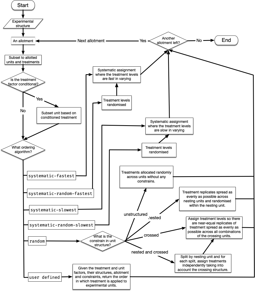
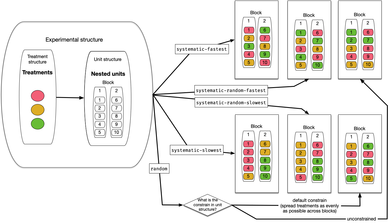
There are five in-built assignment algorithms: “systematic-fastest” (synonym for “systematic”), “systematic-random-fastest” (synonym for “systematic-random”), “systematic-slowest”, “systematic-random-slowest”, and “random”. The variation in systematic assignment results in repeated ordering with respect to the unit order, without regard to any unit structure. When the number of units is not divisible by the total number of treatments, the earlier treatment levels would have an extra replicate. The “systematic-random-fastest” and “systematic-random-slowest” are systematic variants that ensure equal chances for all treatment levels to obtain an extra replicate by randomising the order of treatment levels before the systematic allocation of treatment to units proceeds. The “fastest” and “slowest” variants determine if treatment levels are fast or slow in varying across order of the unit (slow varying meaning that the same treatment levels will be closer together in unit order, whereas fast varying means the same treatment levels are spread out in unit order). An example, with three treatments allotted to ten units, illustrating the in-built assignment algorithms is shown in Figure 4.
Building on the previously defined structure and allotment, we define an algorithm to assign links between unit and treatment levels using the function assign_trts. Below, we use a systematic ordering for the first allotment (fertilizer to row) then a random ordering for the second allotment (interaction of amount and variety to plot). An optional seed number is provided to ensure the generated design could be reproduced. The generated design is shown in Figure 5 (A).
design1 <- alloted1 %>%
  assign_trts(order = c("systematic", "random"),
              seed = 2023) %>%
  serve_table(label_nested = c(row, col))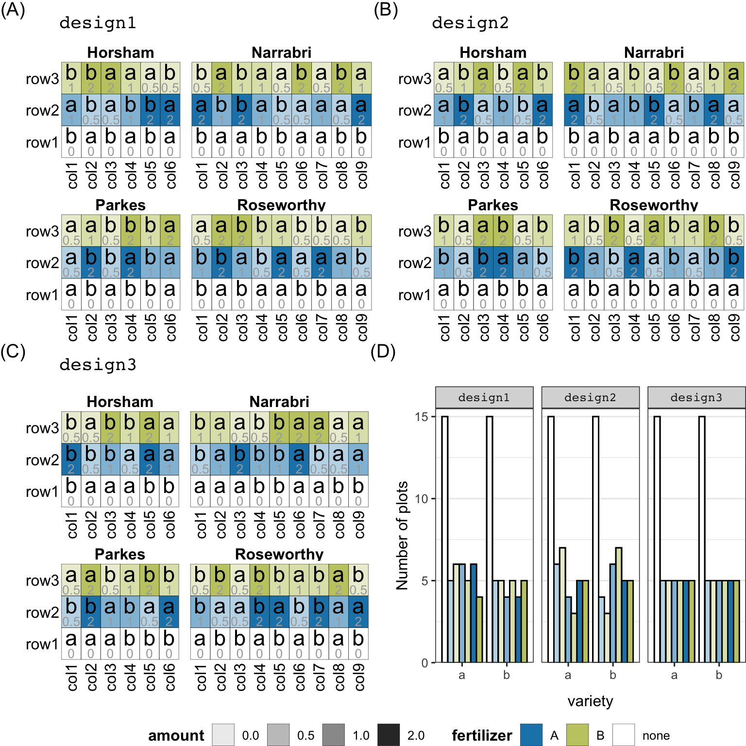
design1, design2, design3). A plot is represented as a tile laid out in a rectangular array for each site. The color of the tile shows the type of fertilizer that the plot was allocated. The opacity of the color represents the amount of fertilizer allocated to the plot (the amount is also written in each tile in grey). The variety (a or b) allocated to the plot is written on each tile. (D) shows the number of plots that were alloted particular level of the treatment for each of the three designs.
While allotment (high-level allocation) and assignment (actual allocation) are distinguished in the system to provide flexibility to the user for defining these processes separately, it is likely that many users would concurrently define these processes. The allot_table function offers a shorthand that combines the call to allot_trts, assign_trts, and serve_table into one call.
To illustrate the difference when treatment interaction is alloted to a unit (like the second allotment in allotment1), below, we have a different allotment where the amount of fertilizer and variety are allotted to plot in a separate allotment. A separate allotment can be assigned using different algorithms and is considered independent of other allotments (unless the treatment factor is conditional on another treatment factor). The resulting assignment is shown in Figure 5 (B) for the design below.
design2 <- (complexd + factrtc) %>%
  allot_table(fertilizer ~ row,
                  amount ~ plot,
                 variety ~ plot,
              order = c("systematic", "random", "random"),
              label_nested = c(row, col),
seed = 2023)The assignment algorithms in the system use the default constraint, which takes the nesting structure defined in the unit structure (i.e. row is nested in site and plot is crossed by row and column and nested in site). This constraint is used to define the nature of “random” assignment. For example, in the code below, we relax this constraint such that the plot factor is constrained within a row (default was row, col and site), which in turn is contained within the site. This difference in constraints results in a different path in the algorithm (as shown in the overview in Figure 3), which generates the design shown in Figure 5 (C).
design3 <- alloted1 %>%
  assign_trts(order = c("systematic", "random"),
              seed = 2023,
              constrain = list(row = "site", plot = "row")) %>%
serve_table(label_nested = c(row, col))The above three different designs (design1, design2 and design3) share the same unit and treatment structure, but the allotment and/or assignment algorithm differed. One result of this is that the treatment replications, as shown in Figure 5 (D), differ across the generated designs with the most ideal distribution seen in design3 (if all fertilizer and amount combinations are of equal interest and fertilizer allocation is restricted to the row; arguably, it is better to remove the latter constraint, if practically feasible, so the units with the control treatment can be assigned for other treatment levels to obtain a more even distribution). The difference in design1 and design2 is that the amount and variety were allocated as an interaction in the former but independently in the latter. The latter process does not ensure near-equal replication of the treatment levels, so it is not surprising that in Figure 5 (D), design2 has the least uniform treatment distribution.
Finding or creating the most appropriate assignment algorithm is one of the challenging tasks in the whole workflow. The default algorithm is unlikely to be optimal for the given structure, and the user is encouraged to modify this step to suit their own design. Section 4.2 presents an example of this.
3.5 Records
The values of a record factor is unknown prior to the execution of the experiment; thus, the method used to define it fundamentally differs from other factors. The record factor is defined using set_rcrds with the arguments in the form of record = unit, where record corresponds to user-specified name of the record, and unit corresponds to an existing unit factor. The LHS of the input argument is always a new factor, as it was the case for set_units and set_trts. Multiple record factors can be specified as separate arguments within the same function call as shown below.
record1 <- design1 %>%
  set_rcrds(biomass = plot,
              yield = plot,
rainfall = site)The above specification can be awkwardly lengthy when we expect multivariate data (i.e., multiple responses of the same unit). In this instance, it may be easier to specify the responses as follows.
design1 %>%
  set_rcrds_of(plot = c("biomass", "yield"),
site = "rainfall")In the above specification, the LHS corresponds to an existing unit factor, while the RHS is a character vector where each element corresponds to the name of the record factor. Notice that in this specification, the RHS elements are quoted as they do not yet exist in the design. By contrast, the RHS specification in set_rcrds is unquoted because these factors already exist. Because the intention of the LHS specification is to point to an existing unit factor, it differs from the convention of other functions that prefix with set_. As a signal to the different input structure, the function appends a suffix _of, which is supposed to act as a signal to the user that this is different from other set_ functions.
Record factors generally do not play a role in the assignment of treatments to units; however, they play a critical role in the analysis stage. The specification of these record factors allows for the user’s intention to be explicit. The added benefits also include the encoding of the expected and simulated values, as described in detail next.
3.5.1 Expected values
If the record factors are defined in the design object, like in record1, then the user may specify the expected values of the records. For example, below we specify that biomass is greater than or equal to zero, yield is between 0 and 10, and rainfall is a factor with two levels: high or low.
expect1 <- record1 %>%
  expect_rcrds(biomass >= 0,
               yield > 0, yield < 10,
factor(rainfall, levels = c("high", "low")))Once the expected values are encoded, they can be used in various functions. For example, suppose we export this design as below.
export_design(expect1, file = "mydesign.xlsx", overwrite = TRUE)The exported design automatically embeds the data validation in the corresponding cells, as shown in Figure 6.
3.5.2 Simulated values
Another benefit of encoding the expected values of the record factors is that you can do a lazy simulation using autofill_rcrds. This function randomly chooses a simulation scheme (including the variables that influence the record), while ensuring that it keeps to the expected values.
set.seed(2023)
sim1auto <- autofill_rcrds(expect1) The aforementioned lazy simulation is designed for quick diagnostics of planned analytical methods and not for any serious simulation study. For proper simulation schemes, users can freely enter their own schemes using the function simulate_process. In this function, the user defines a series of functions, where each function returns either 1) a vector of the same size as the data or 2) a data.frame of the same row dimension as the data. For 1) the name of the function must correspond to the name of the record factor, and for 2) the name must start with a dot and the column names of the returning object must match the names of the record factors.
In the example below, we define two simulation processes called “yield” and “.multi”. The first simulation process is a function that has arguments that define the variety main effect and combined effect of fertilizer and its amount; the return object is a numeric vector where random noise is added on top of the fixed treatment effects. The second simulation process is a function that simulates yield and biomass from a multivariate normal distribution.
process1 <- expect1 %>%
  simulate_process(
    yield = function(v = c(2, 4),
                     af = c(1, 2.5, 3, 0.5, 1, 5, 0)) {
      veffects <- setNames(v, c("a", "b"))
      afeffects <- setNames(af, c("A:0.5", "A:1", "A:2",
                                  "B:0.5", "B:1", "B:2", "none:0"))
      # must return vector of the same size at the data
      veffects[variety] + afeffects[paste0(fertilizer, ":", amount)] + rnorm(n())
    },

    .multi = function() {
      Sigma <- matrix(c(2, 0.9, 0.9, 1), nrow = 2)
      yveffects <- c("a" = 3, "b" = 9)
      bveffects <- c("a" = 1, "b" = 3)
      res <- cbind(yveffects[variety], bveffects[variety])
      res <- res + mvtnorm::rmvnorm(n(), mean = c(0, 0), sigma = Sigma)
      res <- as.data.frame(res)
      colnames(res) <- c("yield", "biomass")
      # must return a data.frame where the column names match the
      # record factor names and the number of rows match the
      # row dimension of data
      res
    }
)After defining the simulation process, the actual simulation of the record is performed through a call to simulate_rcrds. Below, we simulate the actual records by naming the processes we want to use along with any parameters of the function. Optionally, users can define values to censor the simulated values if they lie outside the expected values.
sim1default <- simulate_rcrds(process1, yield = with_params())
sim1var <- simulate_rcrds(process1,
                          yield = with_params(v = c(-1, 5),
                                              .censor = c(0, 10)))
sim1multi <- simulate_rcrds(process1, .multi = with_params(), .seed = 1)
sim1censor <- simulate_rcrds(process1,
                .multi = with_params(.censor = list(yield = c(0, 10),
                                                    biomass = 0)),
.seed = 1)The resulting simulation values from the above calls are shown in Figure 7. We can see in Figure 7 (A) that the sim1auto shows a huge difference in yield with respect to fertilizer type (reflecting that the automated simulation process must have included fertilizer type in the data generation process); sim1default shows some difference in yield across variety (the actual difference is 2 in the simulation process); and sim1var shows a variation in the latter process where the difference in the main variety effects are now more pronounced (actual difference is 6). Figure 7 (B) shows the simulation results from sim1multi and sim1censor; the difference in the latter is that the values are censored to 0 or 10 in the yield and 0 in biomass (the extra points in yield at 0 and 10, and biomass at 0 are easily seen in the plot).
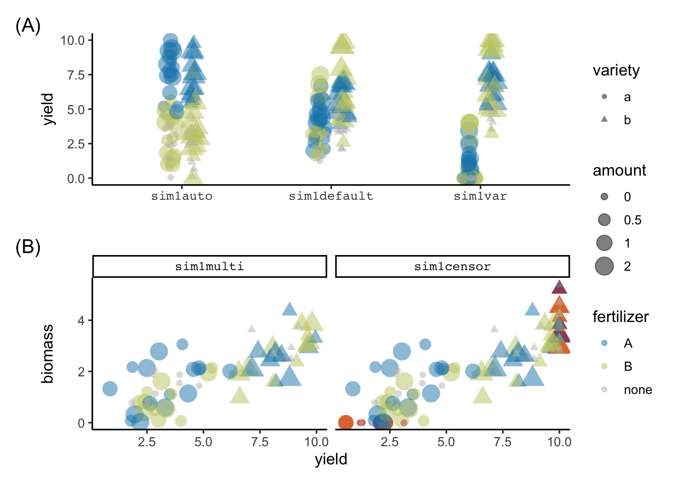
sim1auto, sim1default and sim1var colored by fertilizer type with shape showing the variety, and size reflecting the amount of fertilizer. (B) show the scatterplot of biomass and yield from sim1multi and sim1censor. The only difference in the two simulated values are the censored values that are shown as red points in sim1censor.
4 Worked examples
In addition to the example presented in Section 2, we demonstrate two examples from real experiments: one in ecology and one in linguistics.
4.1 Common garden design
Cochrane et al. (2015) studied the temperature and moisture impact on seedling emergence in a common garden. Below is a digest of the experimental design description.
Example 2: Common garden design
Twelve shelters were constructed on site to manipulate water availability and assess the effects on seed germination, seedling emergence, and seedling growth and survival. Two raised garden beds were placed below each shelter. Water was collected from the roof of each shelter and passively irrigated to the garden beds in each of the three water treatments: reduced rainfall R (80% of the total), natural rainfall N (100% of the total), and increased rainfall I (140% of the total). Each shelter contained one garden bed fitted with 24 warming chambers (W), and one garden bed without warming chambers (C).
Four non-sprouting, obligate seeding species (Banksia media, Banksia coccinea, Banksia baxteri, and Banksia quercifolia) were chosen for the study. Six discrete populations of each species were selected to represent a rainfall cline (High, Medium or Low). The term ‘population’ is used to describe plants originating from a particular geographic and climatic location.
The experimental units were arranged within each garden bed in a balanced array of three columns and eight rows, with seeds from all 24 populations sown in each garden bed. Each row contained seeds from a single species. Each column in the array contained seeds from eight populations corresponding to a particular level of rainfall. Within these constraints, the populations were divided into two sets of 12, so that the same 12 populations always occurred together in a set of four rows.
The allocation of seeds to the experimental units was fully randomised, subject to the constraints of the design.
Based on the above description, my understanding of the unit structure was follows.
garden_units1 <- design("Common garden experiment") %>%
  set_units(shelter = 12,
            bed = nested_in(shelter, 2),
            row = nested_in(bed, 8),
            col = nested_in(bed, 3),
plot = nested_in(bed, crossed_by(row, col)))Initially, I did not understand the full treatment structure and wrote only partial treatment factors. From a further dissection of the description, I inferred that rainfall was the other treatment condition. At this point it was unclear to me how their so-called “population” is actually mapped to the rainfall and so I ignore it for the moment.
garden_trts1 <- set_trts(water = c("R", "N", "I"),
                         chamber = c("W", "C"),
                         species = c("media", "coccinea",
                                     "baxteri", "quercifolia"),
rainfall = c("High", "Medium", "Low"))Based on the description, I inferred the following mapping between the treatment factors to unit factors. The default treatment assignment uses the nesting structures to define the constraint and allocates using the “random” order. A random generation of this design is shown in Figure 8.
garden_design1 <- (garden_units1 + garden_trts1) %>%
  allot_table(water ~ shelter,
              chamber ~ bed,
              species ~ row,
              rainfall ~ col,
              label_nested = c(row, col),
              seed = 2023)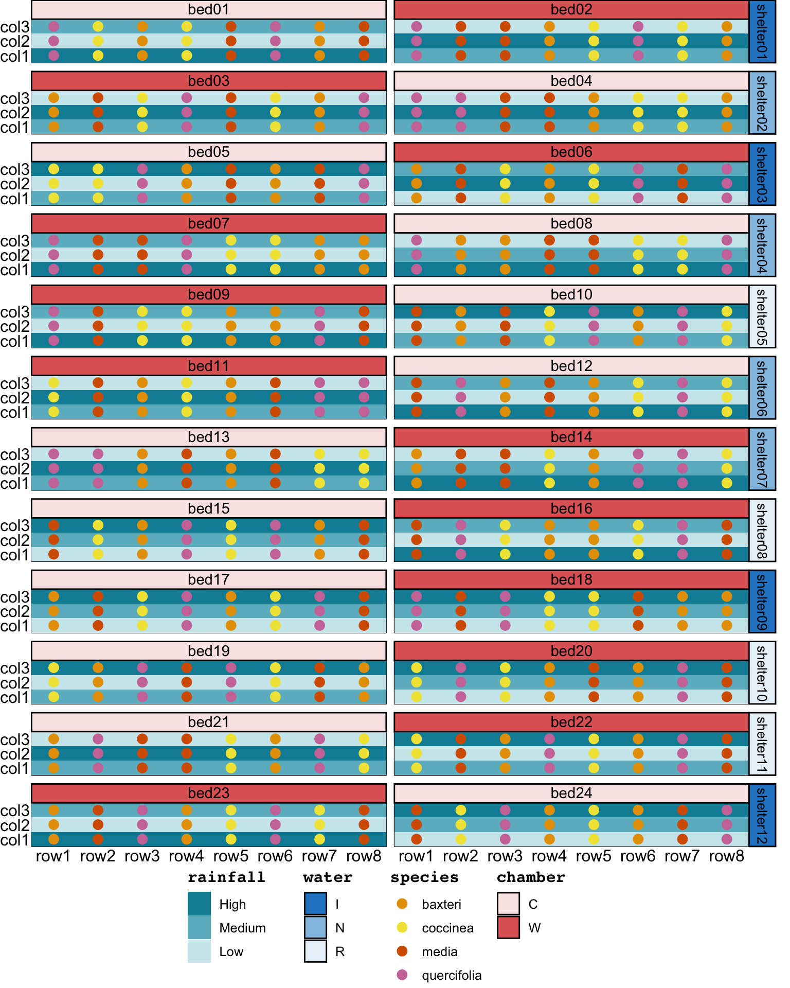
garden design1.
The design above does not necessarily ensure that “the same 12 populations always occurred together in a set of four rows”. This split by four rows sounded like the bed was blocked into two parts across the rows. Below, we create a block factor with two levels in each bed, then the block is assigned to rows in a systematic manner.
garden_units2 <- garden_units1 %>%
  set_units(block = nested_in(bed, 2)) %>%
  allot_units(block ~ row) %>%
assign_units(order = "systematic-slowest")Table A1 in the supplementary material in Cochrane et al. (2015) provides a list of the population IDs. Upon inspection of these IDs, it became clear that they were encoded by species, rainfall cline, and replicate number (e.g., “Bm H1”, “Bm H2”, and “Bm L1” are population of species Banksia media from site with mean annual precipitation of 574, 557, and 301, respectively). There were two replicates for each species and the rainfall cline.
garden_trts2 <- garden_trts1 %>%
set_trts(rep = 1:2)Although not specified in the description, the replicate number was likely allotted to the blocks. The population is then determined from the species, rainfall, and replication number assigned. This assignment ensures that “the same 12 populations always occurred together in a set of four rows”. The resulting design, shown in Figure 9, now aligns with all of the text description.
garden_design2 <- (garden_units2 + garden_trts2) %>%
  allot_table(water ~ shelter,
              chamber ~ bed,
              species ~ row,
              rainfall ~ col,
              rep ~ block, # The missing allotment in garden_design1
              label_nested = c(col, row),
              seed = 2023) %>%
  dplyr::mutate(population = paste0("B", substr(species, 1, 1), " ",
                                    substr(rainfall, 1, 1), rep))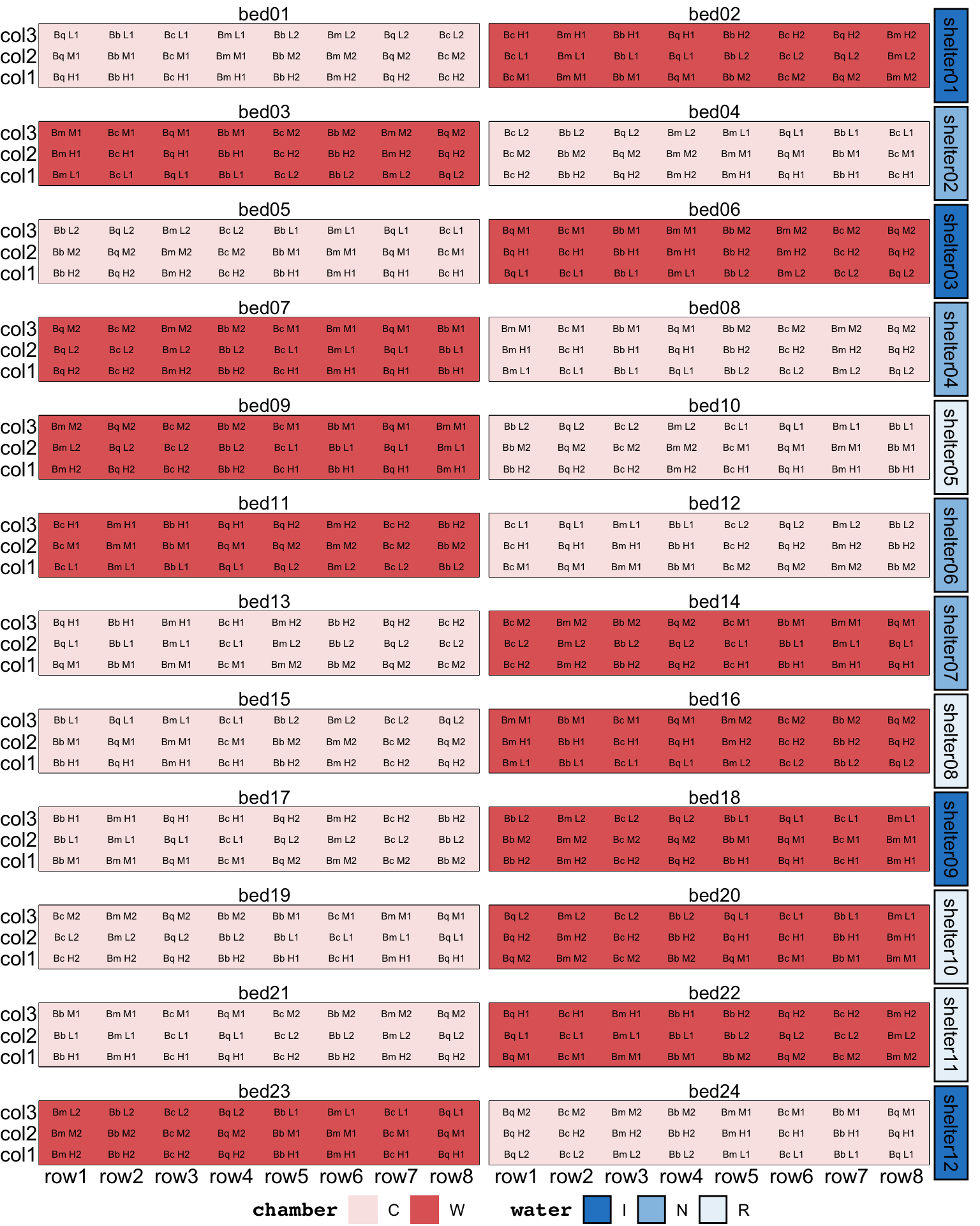
garden design2. The text label in the tile correpond to the population ID in the supplementary material in Cochrane et al. (2015).
4.2 Evaluation of Japanese compositions
E. R. Williams et al. (2021) describe a study on the evaluation of Japanese language compositions written by Japanese beginners by assessors of different backgrounds. The background of this experiment is given in Imaki (2014), with a reduced summary provided below.
Example 3: Evaluation of Japanese composition
Ten compositions (C1–C10) were conditionally drawn from the Taiyaku Database of the National Institute of the Japanese Language on a topic about “special event in my country”. The compositions were selected from writers who were Japanese beginners (studied Japanese for less than 300 hours), with a final selection consisting of three compositions each from Singapore, Brazil, Finland, and a single composition from Cambodia. The selected compositions have an average of 600 characters.
The study investigated the ratings from people of three different backgrounds: native Japanese-language teachers (NT), non-native Japanese language teachers (NNT), and native Japanese who are not language teachers (NG). While it was intended to involve 10 raters from each category, availability resulted in 10, 8, and 11 raters, respectively.
Each rater was asked to evaluate the 10 compositions in four aspects (accuracy, structure and form, context, and richness) plus an overall score. Each rater was asked to rate the composition in a particular order (but different order across raters). The raters were given the option of taking breaks during the assessment process.
Possible carry-over effect was accounted for by using a set of three different \(10 \times 10\) Williams Latin squares design (E. Williams 1949) where the columns represent the raters and the rows represents the order of composition presented. As there were 29 raters, one column was not used.
From the description of the experiment, I inferred the following structure.
composition_str <- design("Japanese composition") %>%
  set_units(background = c("NT", "NNT", "NG"),
            rater = nested_in(background,
                              "NT" ~ 10,
                              "NNT" ~ 8,
                              "NG" ~ 11),
            order = 1:10,
            assess = crossed_by(rater, order)) %>%
  set_trts(composition = paste0("C", 1:10)) %>%
  set_rcrds_of(assess = c("accuracy", "structure", "context",
                          "richness", "overall")) %>%
allot_trts(composition ~ assess)The algorithms in edibble does not contain an algorithm to generate a Williams Latin square design (E. Williams 1949), thus we require a custom treatment assignment order algorithm. The crossdes package (Sailer 2022) has the function williams to generate the Williams Latin squares design; we leverage this function in the algorithm.
In edibble, a custom treatment assignment order algorithm is implemented as an S3 generic function, order_trts, within assign_trts. A new algorithm is created by writing an S3 method as a function with an argument that takes in the name of the algorithm, treatments table, units table, any constraint on the unit that the treatment is applied, and other objects (such as the provenance object that contains the entire graph structure). Suppose we name our new algorithm as “williams” then we can write the S3 method order_trts.williams as follows.
order_trts.williams <- function(name, trts_table, units_table, constrain, ...) {
  # the experimental unit must be a unit crossed by two unit factors
  stopifnot(length(constrain)==2)
  ntrts <- nrow(trts_table)

  # assumes unit is ordered correctly
  units <- lapply(units_table[as.character(constrain)], unique)
  nunits <- sapply(units, length)

  # smaller unit is assumed to be row, larger unit is the column
  unit_row <- as.character(constrain[order(nunits)==1])
  unit_col <- as.character(constrain[order(nunits)==2])

  # the row unit must be exactly equal to the number of treatments
  stopifnot(sort(nunits)[1] == ntrts)

  # generate the William's Latin square design
  williams_design <- t(crossdes::williams(ntrts))

  # number of times to replicate William's design
  nwilliams <- ceiling(sort(nunits)[2]/ntrts)

  # randomise treatment for each replicate
  out <- do.call(rbind, lapply(1:nwilliams, function(i) {
    data.frame(..trt.. = sample(1:ntrts)[as.vector(williams_design)],
               ..row.. = as.vector(row(williams_design)),
               ..col.. = as.vector(col(williams_design)) + (i - 1) * ntrts)
  })) %>%
    subset(..col.. <= sort(nunits)[2])

  # translate row and column to their unit ids
  out[[unit_row]] <- units[[unit_row]][out$..row..]
  out[[unit_col]] <- units[[unit_col]][out$..col..]

  # combine and return the allocated treatment id vector
  # ensuring the treatment order matches the units_table
  units_table$..id.. <- 1:nrow(units_table)
  out <- merge(units_table, out)
  out[order(out$..id..), "..trt..", drop = TRUE]
}The above algorithm is used by setting the argument order = "williams". The above function contains checks to ensure the experimental structure is as expected before proceeding to the allocation. This check makes it clear what the expected experimental structure is for the selected ordering algorithm. The resulting design is illustrated in Figure 10.
composition_design <- composition_str %>%
  assign_trts(order = "williams", seed = 2023) %>%
  serve_table()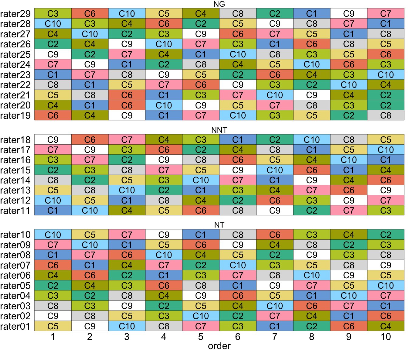
5 Comparisons with other packages
There are currently 103 R-packages in the CRAN Task View of Design of Experiments and Analysis of Experimental Data (as of 2023-11-17). The list is a comprehensive, although not exhaustive, list of R-packages that can construct experimental designs, and some included in the list have an analytical focus or serve as a repository of experimental data (Tanaka and Amaliah 2022).
The packages used to construct experimental designs can be broadly categorised into three approaches: specialist, recipe or general purpose. The first type is exclusive to a domain or has a limited experimental structure. The second often makes use of named experimental designs, e.g., the agricolae package (de Mendiburu 2023) specifies a Latin square design and a split-plot design by the function design.lsd and design.split, respectively. Alternatively, a package can contain a catalogue of pre-optimised designs, e.g., FrF2 (Gromping 2014). The general purpose approach can construct a more flexible range of experimental designs using either a randomisation or optimisation methods. E.g. AlgDesign package (Wheeler 2022) includes a optFederov function finds an optimal design using Federov’s exchange algorithm under certain optimal criterion.
A specialist or recipe approach clearly does not easily allow users to deviate away from a named experimental design. A general purpose approach seems to offer the most flexibility but it often assumes a mise en place; in other words, the ingredients are prepared before “cooking”. A prime example of this is optimal or model-based design, such as in AlgDesign, which requires the initial data structure and specification of the algorithm type and/or model. There are often helper functions to obtain the required initial data structure (such as gen.factorial in AlgDesign).
All of the above mentioned packages have an emphasis on the algorithm to generate the experimental design. On the other hand, edibble package serves as a holistic approach in which segments of the process are modularised. The algorithms, catalogues, or recipes can be integrated into the system as shown in Section 4.2; in this sense, the system is largely complementary to existing systems and offers fundamentally different functionalities. A prime example is the downstream usage of record factors to enter data validation rules (see Section 3.5), which are not offered in the other experimental design packages.
6 Discussion
This paper showcases the capabilities of the edibble package, an implementation of the grammar of experimental designs system by Tanaka (2023) in the R language. While it is conceivable to implement the system in other programming languages, the concrete implementation as an R package should aid in a faster adoption by the scientific community to make their experiments transparent.
The demonstrated downstream benefits of edibble include the ability to specify the record (including responses) of unit factors (set_rcrds), and the expected values these records (expect_rcrds) can take, which in turn can be encoded as data validation rules in the exported data (export_design). These functionalities are also leveraged in the simulation of record factors (simulate_rcrds), including in a lazy, automated fashion (autofill_rcrds). These functionalities aid in better planning and management, and consequently, in the workflow for constructing the experimental design.
Software packages for experimental designs often focus on the algorithmic components of the design. In contrast, edibble package reframes the specification of the experimental design by conceiving experimental designs as a mutable object that can be progressively built. This reframing allows separation in the process of specifying the experimental structure and the assignment algorithm. The benefit of this approach is that users can easily consider various assignment algorithms without respecifying their structure. This approach also aligns with the common mantra that a good experimental design considers the structure first rather than just selecting a recipe design from the menu (Bailey 2008).
Mead, Gilmour, and Mead (2012) attest Procrustean designs that compromise the experimental objective are still common. The edibble package takes a holistic approach that aims to encourage users to think of the experimental structure. By engaging user cognition, this can potentially translate into a better practice of experimental design.
The edibble package can also aid in the teaching of experimental design. Smucker et al. (2023) found from their survey of experimental design courses that nearly all cover randomisation, replication, blocking design principles, and multi-factor experiments, and the use of software for both instruction and assessment is ubiquitous. By adhering closely to the principles of tidyverse (Wickham et al. 2019), which has widespread adoption in modern day practice and teaching (Çetinkaya-Rundel et al. 2022), edibble can integrate more easily in the workflow of everyday users or learners by leveraging their knowledge in a familiar system.
The edibble package is fairly flexible in constructing various fixed experimental structures, and it is fairly easy to wrap existing experimental design algorithms into the system, as shown in Section 4.2. The ability to incorporate other algorithms into the system provides an opportunity for users to select the most appropriate algorithm for their structure. However, there is no guarantee that the generated experimental design will be appropriate or optimal. Afterall, a tool is only as effective as the skillfulness of the hands that wield it. The edibble package aims to cognitively engage the user with the hope that possible broader concerns in the experimental design are detected prior to the execution of the experiment, but ultimately, the user should ensure to perform their own diagnostic checks that the experimental design output is appropriate for their own objectives.
Computational details
The paper was written using Quarto version 1.4.502 with knitr version 1.45, Pandoc version 3.1.1 and R version 4.3.1 (2023-06-16). Some of the figures were drawn using ggplot2 version 3.4.4. The code uses edibble version 1.1.0.
Acknowledgements
I thank Francis Hui and many others that supported the idea and provided feedback on the system.
References
Almende B.V. and Contributors, and Benoit Thieurmel. 2022. visNetwork: Network Visualization Using ’Vis.js’ Library. https://CRAN.R-project.org/package=visNetwork.
Bache, Stefan Milton, and Hadley Wickham. 2022. Magrittr: A Forward-Pipe Operator for r. https://CRAN.R-project.org/package=magrittr.
Bailey, Rosemary A. 2008. Design of Comparative Experiments. Cambridge University Press.
Çetinkaya-Rundel, Mine, Johanna Hardin, Benjamin S. Baumer, Amelia McNamara, Nicholas J. Horton, and Colin Rundel. 2022. “An Educator’s Perspective of the Tidyverse.” Technology Innovations in Statistics Education 14 (1). https://doi.org/10.5070/T514154352.
Cochrane, J. Anne, Gemma L. Hoyle, Colin. J. Yates, Jeff Wood, and Adrienne B. Nicotra. 2015. “Climate Warming Delays and Decreases Seedling Emergence in a Mediterranean Ecosystem.” Oikos 124 (2): 150–60. https://doi.org/10.1111/oik.01359.
de Mendiburu, Felipe. 2023. Agricolae: Statistical Procedures for Agricultural Research. https://CRAN.R-project.org/package=agricolae.
Gromping, Ulrike. 2014. “R Package FrF2 for Creating and Analyzing Fractional Factorial 2-Level Designs.” Journal of Statistical Software 56 (1): 1–56. https://www.jstatsoft.org/v56/i01/.
Hahn, Gerald J. 1984. “Experimental Design in the Complex World.” Technometrics 26 (1): 19–31.
Henry, Lionel, and Hadley Wickham. 2022. Tidyselect: Select from a Set of Strings. https://CRAN.R-project.org/package=tidyselect.
Imaki, Jun. 2014. “Anatomy of Composition: How Are Japanese Compositions Evaluated?” Master’s thesis, Australian National University.
Mead, R, S G Gilmour, and A Mead. 2012. Statistical Principles for the Design of Experiments: Applications to Real Experiments. https://doi.org/10.1017/CBO9781139020879.
Müller, Kirill, and Hadley Wickham. 2023a. Pillar: Coloured Formatting for Columns. https://CRAN.R-project.org/package=pillar.
———. 2023b. Tibble: Simple Data Frames. https://CRAN.R-project.org/package=tibble.
R Core Team. 2023. R: A Language and Environment for Statistical Computing. Vienna, Austria: R Foundation for Statistical Computing. https://www.R-project.org/.
Sailer, Martin Oliver. 2022. Crossdes: Construction of Crossover Designs. https://CRAN.R-project.org/package=crossdes.
Smucker, Byran J., Nathaniel T. Stevens, Jacqueline Asscher, and Peter Goos. 2023. “Profiles in the Teaching of Experimental Design and Analysis.” Journal of Statistics and Data Science Education, June, 1–14. https://doi.org/10.1080/26939169.2023.2205907.
Steinberg, David M, and William G Hunter. 1984. “Experimental Design: Review and Comment.” Technometrics 26 (2): 71–97.
Tanaka, Emi. 2023. “Towards a Unified Language in Experimental Designs Propagated by a Software Framework.” arXiv. https://arxiv.org/abs/2307.11593.
Tanaka, Emi, and Dewi Amaliah. 2022. “Current State and Prospects of R-packages for the Design of Experiments.” arXiv. https://arxiv.org/abs/2206.07532.
Wheeler, Bob. 2022. AlgDesign: Algorithmic Experimental Design. https://CRAN.R-project.org/package=AlgDesign.
Wickham, Hadley, Mara Averick, Jennifer Bryan, Winston Chang, Lucy McGowan, Romain François, Garrett Grolemund, et al. 2019. “Welcome to the Tidyverse.” Journal of Open Source Software 4 (43): 1686. https://doi.org/10.21105/joss.01686.
Wickham, Hadley, Lionel Henry, and Davis Vaughan. 2023. Vctrs: Vector Helpers. https://CRAN.R-project.org/package=vctrs.
Williams, E R, C G Forde, J Imaki, and K Oelkers. 2021. “Experimental Design in Practice: The Importance of Blocking and Treatment Structures.” Australian & New Zealand Journal of Statistics 63 (3): 455–67. https://doi.org/10.1111/anzs.12343.
Williams, Ej. 1949. “Experimental Designs Balanced for the Estimation of Residual Effects of Treatments.” Australian Journal of Chemistry 2 (2): 149. https://doi.org/10.1071/CH9490149.
Wright, Kevin. 2022. Agridat: Agricultural Datasets. https://CRAN.R-project.org/package=agridat.