Neural network II - table of contents

• 
  ETC3250/5250
  • Neural network II
• Acknowledgement
• Wide and deep neural networks
  • Neural network layers
  • Wide neural network
  • Deep neural network
• Feed forward neural networks
  • Mathematical notation
  • Forward evaluation
  • Forward evaluation
  • Forward evaluation
  • Forward evaluation
  • Forward evaluation
  • Forward evaluation
  • Forward evaluation
  • Forward evaluation
  • Forward evaluation
  • Forward evaluation
  • Forward evaluation
  • General feed forward neural network
• Calibration
  • Calibration
  • Regression loss
  • Binary classification loss
  • Multi-class classification loss
  • Optimisation
  • Illustrative example
  • Finding the zero slope
  • Optimising a multi-variable function
  • Searching for the optimal value
  • Illustrative example: Step 0
  • Illustrative example: Step 1
  • Illustrative example: Step 2
  • Illustrative example: Step 3
  • Illustrative example: Step 4
  • Illustrative example: Step 20
  • Gradient descent
  • Limitations of gradient descent
• Stochastic gradient descent
  • Stochastic gradient descent
  • Batch illustration
  • Epoch
  • Epoch
  • Epoch
  • Epoch
  • Epoch
  • Epoch
  • Epoch
  • Backpropagation
  • Vanishing gradient problem
• An application to fashion MNIST data
  • Fashion MNIST data
  • Neural network in R 1 prepare the data
  • Neural network in R 2 Define architechture
  • Neural network in R 3 Choose loss function
  • Neural network in R 4 Fit model
  • Model diagnostic
  • Predicting from neural network
  • Visually checking the prediction: observation 1
  • Visually checking the prediction: observation 2
  • Visually checking the prediction: observation 3
  • Visually checking the prediction: observation 4
  • Visually checking the prediction: observation 5
• Limitations
  • Cons of neural network
• Takeaways

ETC3250/5250

Introduction to Machine Learning

Neural network II

Lecturer: Emi Tanaka

Department of Econometrics and Business Statistics

Acknowledgement

This lecture benefited from the lecture notes by Dr. Ruben Loaiza-Maya.

Wide and deep neural networks

Neural network layers

• The neural network we saw last week had 3 layers:
  • Input layer (2 nodes)
  • Middle or hidden layer (3 nodes)
  • Output layer (3 nodes)

• The number of nodes in the input and output layer are constrained by the input data and desired output (regression or classification).

Wide neural network

• We refer to neural network with large number of neurons (nodes) in the hidden layer as a wide neural network.
• The number of parameters in the neural network model generally increases exponentially as the number of neurons increase.
• Wide neural networks are however harder to calibrate as the number of neurons increase.

Here, the addition of 2 neurons increases the number of parameters by 10.

Deep neural network

• Deep neural networks, also called feed forward neural networks, add more layers.
• The number of parameters also can increase exponentially.
• But it can achieve flexibility with less neuron and it can be faster to calibrate.

Feed forward neural networks

Mathematical notation

• We now use a new mathematical notation for neural networks:
  • L denotes the total number of layers,
  • a^{(l)}_k denotes the value for layer l for k-th node,
  • K_l denotes the total number of nodes in layer l,
  • h_l denotes the activation function in layer l,
  • b_k^{(l)} denotes the bias in node k of layer l,
  • \boldsymbol{w}_k^{(l)} denotes the weights for k-th node of layer l.

Forward evaluation

Input layer

\boldsymbol{x} = (1, x_1)^\top

Forward evaluation

Input layer

\boldsymbol{x} = (1, x_1)^\top

Layer 2

• The activation function h_2 is ReLU.
• a^{(2)}_1 = h_2(\boldsymbol{\beta}_1^\top\boldsymbol{x})

Forward evaluation

Input layer

\boldsymbol{x} = (1, x_1)^\top

Layer 2

• The activation function h_2 is ReLU.
• a^{(2)}_1 = h_2(\boldsymbol{\beta}_1^\top\boldsymbol{x}), a^{(2)}_2 = h_2(\boldsymbol{\beta}_2^\top\boldsymbol{x})

Forward evaluation

Input layer

\boldsymbol{x} = (1, x_1)^\top

Layer 2

• The activation function h_2 is ReLU.
• a^{(2)}_1 = h_2(\boldsymbol{\beta}_1^\top\boldsymbol{x}), a^{(2)}_2 = h_2(\boldsymbol{\beta}_2^\top\boldsymbol{x}), a^{(2)}_3 = h_2(\boldsymbol{\beta}_3^\top\boldsymbol{x})

Forward evaluation

Input layer

\boldsymbol{x} = (1, x_1)^\top

Layer 2

• The activation function h_2 is ReLU.
• a^{(2)}_1 = h_2(\boldsymbol{\beta}_1^\top\boldsymbol{x}), a^{(2)}_2 = h_2(\boldsymbol{\beta}_2^\top\boldsymbol{x}), a^{(2)}_3 = h_2(\boldsymbol{\beta}_3^\top\boldsymbol{x})
• \boldsymbol{a}^{(2)} = (a^{(2)}_1, a^{(2)}_2, a^{(2)}_3)^\top

Forward evaluation

Input layer

\boldsymbol{x} = (1, x_1)^\top

Layer 2

• The activation function h_2 is ReLU.
• a^{(2)}_1 = h_2(\boldsymbol{\beta}_1^\top\boldsymbol{x}), a^{(2)}_2 = h_2(\boldsymbol{\beta}_2^\top\boldsymbol{x}), a^{(2)}_3 = h_2(\boldsymbol{\beta}_3^\top\boldsymbol{x})
• \boldsymbol{a}^{(2)} = (a^{(2)}_1, a^{(2)}_2, a^{(2)}_3)^\top

Layer 3

• The activation function h_3 is Tanh.
• a^{(3)}_1 = h_2(b_1^{(3)}+\boldsymbol{w}_1^{(3)\top}\boldsymbol{a}^{(2)})

Forward evaluation

Input layer

\boldsymbol{x} = (1, x_1)^\top

Layer 2

• The activation function h_2 is ReLU.
• a^{(2)}_1 = h_2(\boldsymbol{\beta}_1^\top\boldsymbol{x}), a^{(2)}_2 = h_2(\boldsymbol{\beta}_2^\top\boldsymbol{x}), a^{(2)}_3 = h_2(\boldsymbol{\beta}_3^\top\boldsymbol{x})
• \boldsymbol{a}^{(2)} = (a^{(2)}_1, a^{(2)}_2, a^{(2)}_3)^\top

Layer 3

• The activation function h_3 is Tanh.
• a^{(3)}_1 = h_3(b_1^{(3)}+\boldsymbol{w}_1^{(3)\top}\boldsymbol{a}^{(2)}), a^{(3)}_2 = h_3(b_2^{(3)}+\boldsymbol{w}_2^{(3)\top}\boldsymbol{a}^{(2)})

Forward evaluation

Input layer

\boldsymbol{x} = (1, x_1)^\top

Layer 2

• The activation function h_2 is ReLU.
• a^{(2)}_1 = h_2(\boldsymbol{\beta}_1^\top\boldsymbol{x}), a^{(2)}_2 = h_2(\boldsymbol{\beta}_2^\top\boldsymbol{x}), a^{(2)}_3 = h_2(\boldsymbol{\beta}_3^\top\boldsymbol{x})
• \boldsymbol{a}^{(2)} = (a^{(2)}_1, a^{(2)}_2, a^{(2)}_3)^\top

Layer 3

• The activation function h_3 is Tanh.
• a^{(3)}_1 = h_3(b_1^{(3)}+\boldsymbol{w}_1^{(3)\top}\boldsymbol{a}^{(2)}), a^{(3)}_2 = h_3(b_2^{(3)}+\boldsymbol{w}_2^{(3)\top}\boldsymbol{a}^{(2)})
• \boldsymbol{a}^{(3)} = (a^{(3)}_1, a^{(3)}_2)^\top

Forward evaluation

Input layer

\boldsymbol{x} = (1, x_1)^\top

Layer 2

• The activation function h_2 is ReLU.
• a^{(2)}_1 = h_2(\boldsymbol{\beta}_1^\top\boldsymbol{x}), a^{(2)}_2 = h_2(\boldsymbol{\beta}_2^\top\boldsymbol{x}), a^{(2)}_3 = h_2(\boldsymbol{\beta}_3^\top\boldsymbol{x})
• \boldsymbol{a}^{(2)} = (a^{(2)}_1, a^{(2)}_2, a^{(2)}_3)^\top

Layer 3

• The activation function h_3 is Tanh.
• a^{(3)}_1 = h_3(b_1^{(3)}+\boldsymbol{w}_1^{(3)\top}\boldsymbol{a}^{(2)}), a^{(3)}_2 = h_3(b_2^{(3)}+\boldsymbol{w}_2^{(3)\top}\boldsymbol{a}^{(2)})
• \boldsymbol{a}^{(3)} = (a^{(3)}_1, a^{(3)}_2)^\top

Output layer

• The activation function h_4 is Softmax.
• f_1(\boldsymbol{x}) = h_4(b_1^{(4)}+\boldsymbol{w}_1^{(4)\top}\boldsymbol{a}^{(3)})

Forward evaluation

Input layer

\boldsymbol{x} = (1, x_1)^\top

Layer 2

• The activation function h_2 is ReLU.
• a^{(2)}_1 = h_2(\boldsymbol{\beta}_1^\top\boldsymbol{x}), a^{(2)}_2 = h_2(\boldsymbol{\beta}_2^\top\boldsymbol{x}), a^{(2)}_3 = h_2(\boldsymbol{\beta}_3^\top\boldsymbol{x})
• \boldsymbol{a}^{(2)} = (a^{(2)}_1, a^{(2)}_2, a^{(2)}_3)^\top

Layer 3

• The activation function h_3 is Tanh.
• a^{(3)}_1 = h_3(b_1^{(3)}+\boldsymbol{w}_1^{(3)\top}\boldsymbol{a}^{(2)}), a^{(3)}_2 = h_3(b_2^{(3)}+\boldsymbol{w}_2^{(3)\top}\boldsymbol{a}^{(2)})
• \boldsymbol{a}^{(3)} = (a^{(3)}_1, a^{(3)}_2)^\top

Output layer

• The activation function h_4 is Softmax.
• f_1(\boldsymbol{x}) = h_4(b_1^{(4)}+\boldsymbol{w}_1^{(4)\top}\boldsymbol{a}^{(3)}), f_2(\boldsymbol{x}) = h_4(b_2^{(4)}+\boldsymbol{w}_2^{(4)\top}\boldsymbol{a}^{(3)})

Forward evaluation

Input layer

\boldsymbol{x} = (1, x_1)^\top

Layer 2

• The activation function h_2 is ReLU.
• a^{(2)}_1 = h_2(\boldsymbol{\beta}_1^\top\boldsymbol{x}), a^{(2)}_2 = h_2(\boldsymbol{\beta}_2^\top\boldsymbol{x}), a^{(2)}_3 = h_2(\boldsymbol{\beta}_3^\top\boldsymbol{x})
• \boldsymbol{a}^{(2)} = (a^{(2)}_1, a^{(2)}_2, a^{(2)}_3)^\top

Layer 3

• The activation function h_3 is Tanh.
• a^{(3)}_1 = h_3(b_1^{(3)}+\boldsymbol{w}_1^{(3)\top}\boldsymbol{a}^{(2)}), a^{(3)}_2 = h_3(b_2^{(3)}+\boldsymbol{w}_2^{(3)\top}\boldsymbol{a}^{(2)})
• \boldsymbol{a}^{(3)} = (a^{(3)}_1, a^{(3)}_2)^\top

Output layer

• The activation function h_4 is Softmax.
• f_1(\boldsymbol{x}) = h_4(b_1^{(4)}+\boldsymbol{w}_1^{(4)\top}\boldsymbol{a}^{(3)}), f_2(\boldsymbol{x}) = h_4(b_2^{(4)}+\boldsymbol{w}_2^{(4)\top}\boldsymbol{a}^{(3)}), f_3(\boldsymbol{x}) = h_4(b_3^{(4)}+\boldsymbol{w}_3^{(4)\top}\boldsymbol{a}^{(3)})

General feed forward neural network

• Input layer: \boldsymbol{x} = (1, x_1, \dots, x_p)^\top
• Layer 2: \boldsymbol{a}^{(2)} = (h_2(\boldsymbol{\beta}^\top_1\boldsymbol{x}), \dots, h_2(\boldsymbol{\beta}^\top_{K_2}\boldsymbol{x}))^\top
• Layer 3: \boldsymbol{a}^{(3)} = (h_3(b_1^{(3)}+\boldsymbol{w}^{(3)\top}_1\boldsymbol{a}^{(2)}), \dots, h_3(b_{K_3}^{(3)}+\boldsymbol{w}^{(3)\top}_{K_3}\boldsymbol{a}^{(2)}))^\top
• \cdots
• Layer l:\boldsymbol{a}^{(l)} = (h_l(b_1^{(l)}+\boldsymbol{w}^{(l)\top}_1\boldsymbol{a}^{(l - 1)}), \dots, h_l(b_{K_l}^{(l)}+\boldsymbol{w}^{(l)\top}_{K_l}\boldsymbol{a}^{(l-1)}))^\top
• \cdots
• Layer L -1: \boldsymbol{a}^{(L-1)} = (h_{L-1}(b_1^{(L-1)}+\boldsymbol{w}^{(L-1)\top}_1\boldsymbol{a}^{(L-2)}), \dots, h_{L-1}(b_{K_{L-1}}^{({L-1})}+\boldsymbol{w}^{({L-1})\top}_{K_{L-1}}\boldsymbol{a}^{(L-2)}))^\top
• Output layer: f_k(\boldsymbol{x}) = h_L(b^{(L)}+\boldsymbol{w}_k^{(L)\top}\boldsymbol{a}^{(L-1)}).

• The output actually depends on the parameters: \boldsymbol{\theta} = (\underbrace{\beta_1, \dots, \beta_{K_2}}_{\text{coefficients}}, \underbrace{b_1^{(3)}, \dots, b_{K_{L-1}}^{(L-1)}}_{\text{biases}},\underbrace{\boldsymbol{w}_1^{(3)\top}, \dots, \boldsymbol{w}_k^{(L)\top}}_{\text{weights}})^\top.
• We can write this dependency more explicitly as f_k(\boldsymbol{x}~|~\boldsymbol{\theta}).

• How do we calibrate (or train) these parameters \boldsymbol{\theta}?

Calibration

Calibration

• As like other models, we:
  • define a loss function, and
  • find parameters that minimise this loss function.
• What loss function we use depends on the problem.

Regression loss

• Find \boldsymbol{\theta} that minimises the mean squared error:

\text{MSE}(\boldsymbol{\theta}) = \frac{1}{n}\sum_{i=1}^n\left(y_i - f(\boldsymbol{x}_i~|~\boldsymbol{\theta})\right)^2

Binary classification loss

• Find \boldsymbol{\theta} that minimises the binary cross-entropy (BCE):

\text{BCE}(\boldsymbol{\theta}) = -\frac{1}{n}\sum_{i=1}^n\left\{y_i\log(P(y_i=1~|~\boldsymbol{x}_i,\boldsymbol{\theta})) + (1-y_i)\log(1 - P(y_i=1~|~\boldsymbol{x}_i,\boldsymbol{\theta}))\right\}

Multi-class classification loss

• Find \boldsymbol{\theta} that minimises the cross-entropy (CE):

\text{CE}(\boldsymbol{\theta}) = -\frac{1}{n}\sum_{i=1}^n\sum_{j=1}^my_{ij}\log(P(y_{ij} = 1~|~\boldsymbol{x}_i,\boldsymbol{\theta}))

Optimisation

• Regardless of whether it is regression or classification, we must find hyperparameters that optimise a loss function.
• Finding these hyperparameters is often hard with no closed-form solution.
• There are various optimisation methods to find these hyperparameters – we discuss:
  • gradient descent, and
  • stochastic gradient descent.

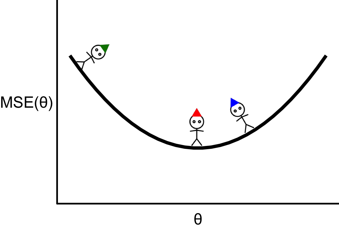
Illustrative example

• Suppose that we have a regression problem that require callibration of one hyperparameter with MSE loss function.

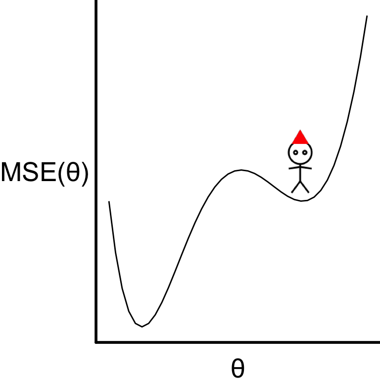
• Our goal is to find \theta that corresponds to the bottom of the curve.

Finding the zero slope

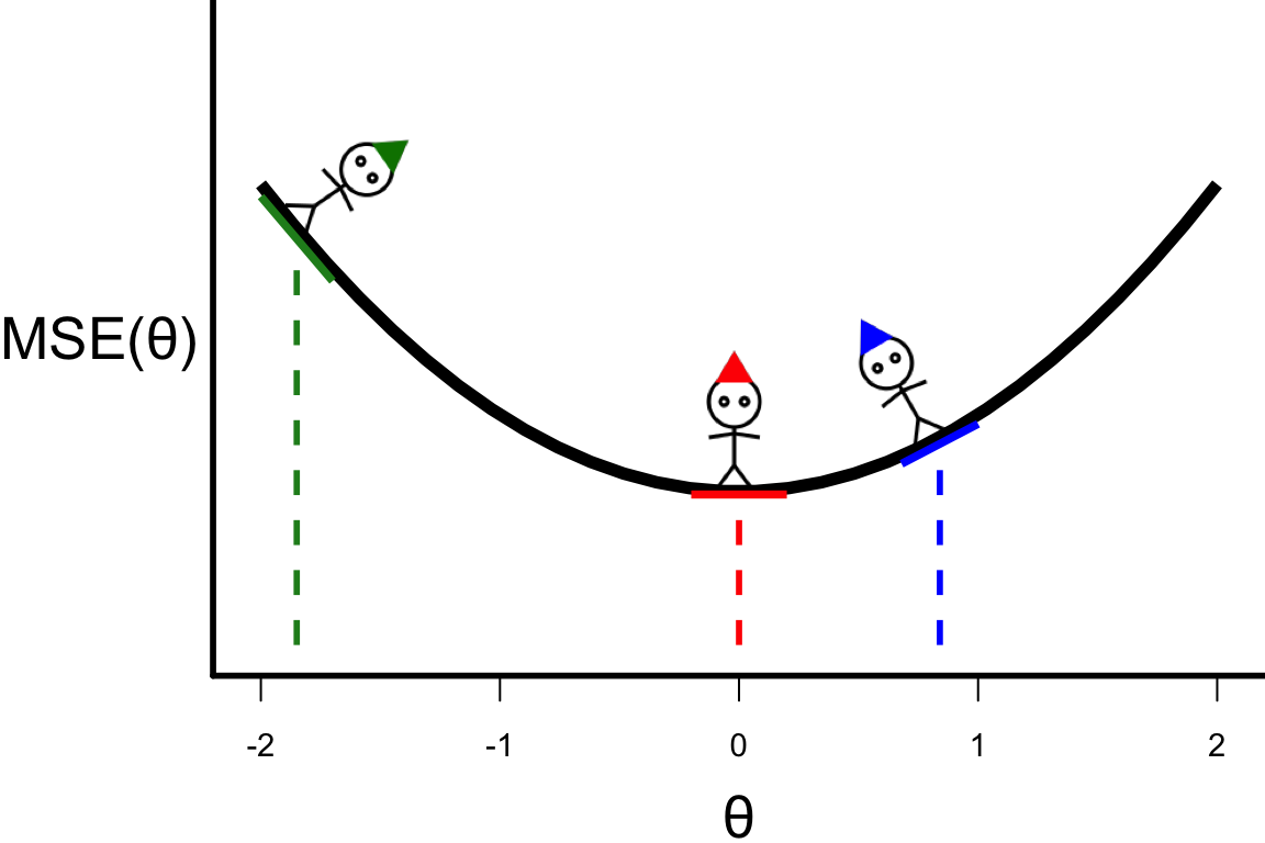
• Suppose that we calculate \text{MSE}(\theta) for three values of \theta.
• For this function, the optimal \theta is where the individual with the red hat is.
• This is also where the slope (or derivative) is zero: \frac{\partial \text{MSE}(\theta)}{\partial \theta} = 0.

Optimising a multi-variable function

• In practice, \boldsymbol{\theta} is typically a vector of length d with d > 1.
• The optimal value of \boldsymbol{\theta} is then found by solving for \boldsymbol{\theta} such that \nabla \text{MSE}(\boldsymbol{\theta}) = 0 where \nabla \text{MSE}(\boldsymbol{\theta}) = \left(\frac{\partial\text{MSE}(\boldsymbol{\theta})}{\partial\theta_1}, \dots, \frac{\partial\text{MSE}(\boldsymbol{\theta})}{\partial\theta_d}\right)^\top is the vector of slopes for all parameters (gradient).
• Finding \boldsymbol{\theta} such that \nabla \text{MSE}(\boldsymbol{\theta}) = 0 is hard!
• We use gradient descent to find this.

Searching for the optimal value

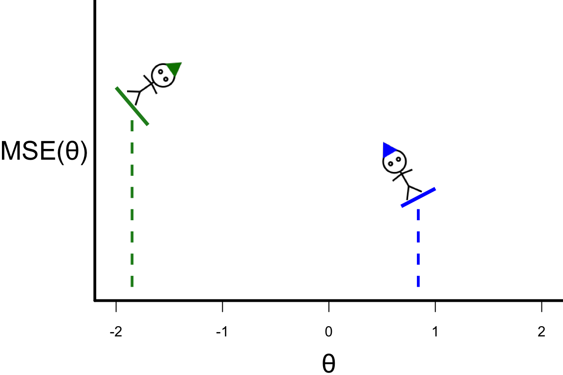
• To search for the optimal value of \theta, we choose some starting points.
• We can calculate the slope at the starting points giving us a guide where to search next: \theta^{[s+1]} = \theta^{[s]} - r \left.\frac{\partial\text{MSE}(\theta)}{\partial\theta}\right\vert_{\theta=\theta^{[s]}}, where r > 0 is the length of the step.

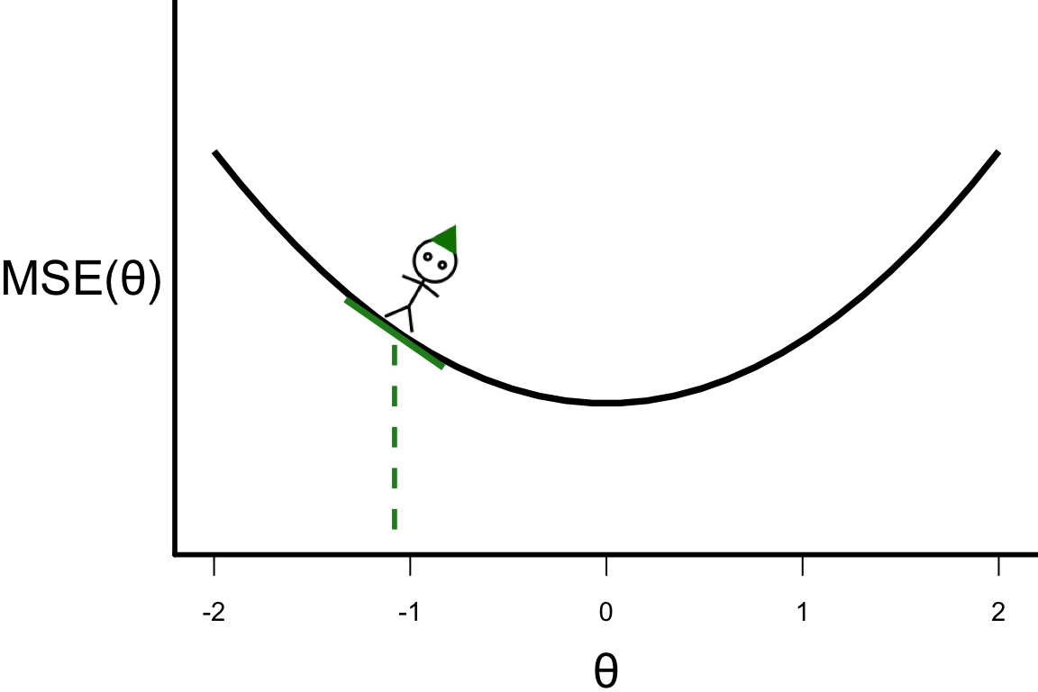
Illustrative example: Step 0

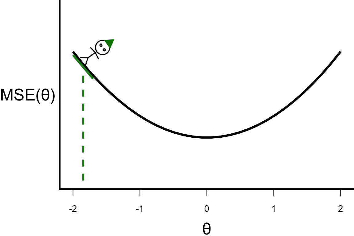
\theta^{[s+1]} = \theta^{[s]} - r \left.\frac{\partial\text{MSE}(\theta)}{\partial\theta}\right\vert_{\theta=\theta^{[s]}}

• Suppose
  • \frac{\partial\text{MSE}(\theta)}{\partial\theta} = 4\theta,
  • r = 0.1, and
  • the starting point \theta^{[0]} = -1.8.

• \theta^{[1]} = -1.8 - 0.1 \times 4 \times (-1.8) = -1.08.

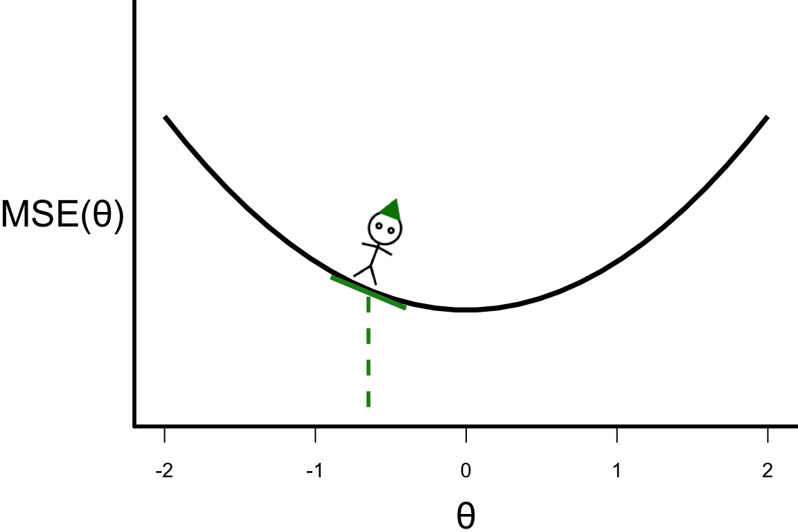
Illustrative example: Step 1

\theta^{[s+1]} = \theta^{[s]} - r \left.\frac{\partial\text{MSE}(\theta)}{\partial\theta}\right\vert_{\theta=\theta^{[s]}}

• \theta^{[1]} = -1.08

• \theta^{[2]} = -1.08 - 0.1 \times 4 \times (-1.08) = -0.648.

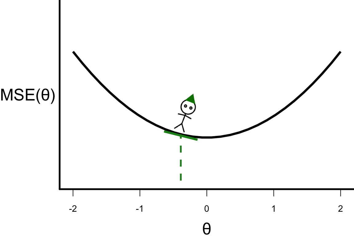
Illustrative example: Step 2

\theta^{[s+1]} = \theta^{[s]} - r \left.\frac{\partial\text{MSE}(\theta)}{\partial\theta}\right\vert_{\theta=\theta^{[s]}}

• \theta^{[2]} = -0.648

• \theta^{[3]} = -0.648 - 0.1 \times 4 \times (-0.648) = -0.3888.

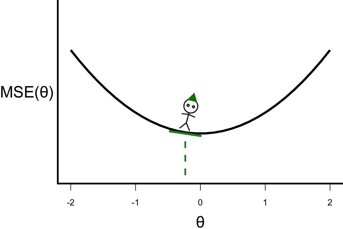
Illustrative example: Step 3

\theta^{[s+1]} = \theta^{[s]} - r \left.\frac{\partial\text{MSE}(\theta)}{\partial\theta}\right\vert_{\theta=\theta^{[s]}}

• \theta^{[3]} = -0.3888

• \theta^{[4]} = -0.3888 - 0.1 \times 4 \times (-0.3888) = -0.23328

Illustrative example: Step 4

\theta^{[s+1]} = \theta^{[s]} - r \left.\frac{\partial\text{MSE}(\theta)}{\partial\theta}\right\vert_{\theta=\theta^{[s]}}

• \theta^{[4]} = -0.23328

• \theta^{[5]} = -0.23328 - 0.1 \times 4 \times (-0.23328) = -0.139968

\cdots

Illustrative example: Step 20

\theta^{[s+1]} = \theta^{[s]} - r \left.\frac{\partial\text{MSE}(\theta)}{\partial\theta}\right\vert_{\theta=\theta^{[s]}}

• \theta^{[20]} = -0.00006581085

• What if there are more than one parameter?

Gradient descent

• In the multi-variable version: \boldsymbol{\theta}^{[s+1]} = \left.\boldsymbol{\theta}^{[s]} - r\nabla \text{MSE}(\boldsymbol{\theta})\right\vert_{\theta=\theta^{[s]}}. where r>0 is the learning rate.
• You need a starting value \boldsymbol{\theta}^{[0]} and take a number of steps.
• This is known as the gradient descent method.

Limitations of gradient descent

• In practice, the loss function generally involves valuation for each observation, e.g. for MSE: \nabla \text{MSE}(\boldsymbol{\theta}) = \frac{1}{n}\sum_{i=1}^n\nabla\left(y_i - f(\boldsymbol{x}_i~|~\boldsymbol{\theta})\right)^2.
• This can be computationally expensive if n is large.
• Gradient descent optimisation can get stuck in local optima.

Stochastic gradient descent

Stochastic gradient descent

• In a stochastic gradient descent (SGD) considers at each step \boldsymbol{\theta}^{[s+1]} = \boldsymbol{\theta}^{[s]} - r \left.\nabla \hat{\text{MSE}}(\boldsymbol{\theta})\right\vert_{\boldsymbol{\theta}=\boldsymbol{\theta}^{[s]}} where \left.\nabla \hat{\text{MSE}}(\boldsymbol{\theta})\right\vert_{\boldsymbol{\theta}=\boldsymbol{\theta}^{[s]}}=\frac{1}{M}\sum_{i\in B^{[s]}}\nabla\left(y_i - f(\boldsymbol{x}_i~|~\boldsymbol{\theta}^{[s]})\right)^2. where B^{[s]} denotes a set of random batch of M \ll n observations at iteration s.

Batch illustration

• Suppose we have n = 1000.
• We draw a (random without replacement) batch of size 3, say resulting in B^{[1]} = \{133, 606, 851\}.
• With gradient descent, \nabla\text{MSE}(\boldsymbol{\theta}) = \frac{1}{1000}\left(\nabla(y_1 - f(\boldsymbol{x}_1~|~\boldsymbol{\theta})^2 + \nabla(y_2 - f(\boldsymbol{x}_2~|~\boldsymbol{\theta})^2 + \cdots + \nabla(y_{1000} - f(\boldsymbol{x}_{1000}~|~\boldsymbol{\theta})^2\right).
• But for stochastic gradient descent, we replace this with: \nabla\hat{\text{MSE}}(\boldsymbol{\theta}) = \frac{1}{3}\left(\nabla(y_{133} - f(\boldsymbol{x}_{133}~|~\boldsymbol{\theta})^2 + \nabla(y_{606} - f(\boldsymbol{x}_{606}~|~\boldsymbol{\theta})^2 + \nabla(y_{851} - f(\boldsymbol{x}_{851}~|~\boldsymbol{\theta})^2\right).
• The latter is faster to calculate and can escape from local optima.

Epoch

• The number of epochs is the number of times that the algorithm has used all observations in the data.
• Illustrative data: y_1, y_2, y_3, y_4, y_5, y_6, y_7, y_8, y_9, y_{10}, y_{11}, y_{12}

Epoch

• The number of epochs is the number of times that the algorithm has used all observations in the data.
• Illustrative data: y_1, y_2, y_3, y_4, y_5, y_6, y_7, y_8, y_9, y_{10}, y_{11}, y_{12}

1. s = 1, B^{[1]} = \color{red}{\{4, 8, 10\}}

Epoch

• The number of epochs is the number of times that the algorithm has used all observations in the data.
• Illustrative data: y_1, y_2, y_3, y_4, y_5, y_6, y_7, y_8, y_9, y_{10}, y_{11}, y_{12}

1. s = 1, B^{[1]} = \{4, 8, 10\}
2. s = 2, B^{[2]} = \color{red}{\{1, 5, 12\}}

Epoch

• The number of epochs is the number of times that the algorithm has used all observations in the data.
• Illustrative data: y_1, y_2, y_3, y_4, y_5, y_6, y_7, y_8, y_9, y_{10}, y_{11}, y_{12}

1. s = 1, B^{[1]} = \{4, 8, 10\}
2. s = 2, B^{[2]} = \{1, 5, 12\}
3. s = 3, B^{[3]} = \color{red}{\{2, 3, 6\}}

Epoch

• The number of epochs is the number of times that the algorithm has used all observations in the data.
• Illustrative data: y_1, y_2, y_3, y_4, y_5, y_6, y_7, y_8, y_9, y_{10}, y_{11} , y_{12}

1. s = 1, B^{[1]} = \{4, 8, 10\}
2. s = 2, B^{[2]} = \{1, 5, 12\}
3. s = 3, B^{[3]} = \{2, 3, 6\}
4. s = 4, B^{[4]} = \color{red}{\{7, 9, 11\}}

Epoch

• The number of epochs is the number of times that the algorithm has used all observations in the data.
• Illustrative data: y_1, y_2, y_3, y_4, y_5, y_6, y_7, y_8, y_9, y_{10}, y_{11} , y_{12}

1. s = 1, B^{[1]} = \{4, 8, 10\}
2. s = 2, B^{[2]} = \{1, 5, 12\}
3. s = 3, B^{[3]} = \{2, 3, 6\}
4. s = 4, B^{[4]} = \{7, 9, 11\}

Epoch 1

Epoch

• The number of epochs is the number of times that the algorithm has used all observations in the data.
• Illustrative data: y_1, y_2, y_3, y_4, y_5, y_6, y_7, y_8, y_9, y_{10}, y_{11} , y_{12}

1. s = 1, B^{[1]} = \{4, 8, 10\}
2. s = 2, B^{[2]} = \{1, 5, 12\}
3. s = 3, B^{[3]} = \{2, 3, 6\}
4. s = 4, B^{[4]} = \{7, 9, 11\}

Epoch 1

5. s = 5, B^{[5]} = \{3, 4, 11\}
6. s = 6, B^{[6]} = \{2, 7, 9\}
7. s = 7, B^{[7]} = \{6, 10, 12\}
8. s = 8, B^{[8]} = \{1, 5, 8\}

Epoch 2

Backpropagation

• In evaluating \nabla \hat{\text{MSE}}(\boldsymbol{\theta}), we must evaluate \nabla (y_i - f(\boldsymbol{x}_i~|~\boldsymbol{\theta}))^2.

• Now we have: \nabla (y_i - f(\boldsymbol{x}_i~|~\boldsymbol{\theta}))^2 = - 2(y_i - f(\boldsymbol{x}_i~|~\boldsymbol{\theta}))\times \underbrace{\frac{\partial f(\boldsymbol{x}_i|\boldsymbol{\theta})}{\partial \boldsymbol{a}_i^{(L - 1)}}}_{\text{Layer }L -1}\times \underbrace{\frac{\partial \boldsymbol{a}_i^{(L - 1)}}{\partial \boldsymbol{a}_i^{(L - 2)}}}_{\text{Layer }L -2}\times \underbrace{\frac{\partial \boldsymbol{a}_i^{(L - 2)}}{\partial \boldsymbol{a}_i^{(L - 3)}}}_{\text{Layer }L -3}\times \cdots \times \underbrace{\frac{\partial \boldsymbol{a}_i^{(2)}}{\partial \boldsymbol{\theta}}}_{\text{Layer }1}.

• The gradient of the later layers is calculated earlier.

• For parameter \theta, we can show \frac{\partial (y_i - f(\boldsymbol{x}_i~|~\boldsymbol{\theta}))^2}{\partial \theta} = \text{constant}\times \underbrace{\frac{\partial h_L(a_i^{(L-1)})}{\partial a_i^{(L-1)}}}_{\text{Layer }L -1}\times \underbrace{\frac{\partial h_L(a_i^{(L-2)})}{\partial a_i^{(L-2)}}}_{\text{Layer }L -2}\times \underbrace{\frac{\partial h_L(a_i^{(L-3)})}{\partial a_i^{(L-3)}}}_{\text{Layer }L -3}\times \cdots \times \underbrace{\frac{\partial h_2(x_i| \theta)}{\partial \theta}}_{\text{Layer }1}.

Vanishing gradient problem

\frac{\partial (y_i - f(\boldsymbol{x}_i~|~\boldsymbol{\theta}))^2}{\partial \theta} = \text{constant}\times \underbrace{\frac{\partial h_L(a_i^{(L-1)})}{\partial a_i^{(L-1)}}}_{\text{Layer }L -1}\times \underbrace{\frac{\partial h_L(a_i^{(L-2)})}{\partial a_i^{(L-2)}}}_{\text{Layer }L -2}\times \underbrace{\frac{\partial h_L(a_i^{(L-3)})}{\partial a_i^{(L-3)}}}_{\text{Layer }L -3}\times \cdots \times \underbrace{\frac{\partial h_2(x_i| \theta)}{\partial \theta}}_{\text{Layer }1}.

• If h_l is the Sigmoid activation function then 0 < \frac{\partial h_l(a_i^{(l -1)})}{\partial a_i^{(l -1)}} < 1.
• If the L is large then this can result in \nabla (y_i - f(\boldsymbol{x}_i | \boldsymbol{\theta}))^2 \approx 0.
• This phenomenon is referred to as the vanishing gradient problem and results in difficulty with calibrating the neural network.
• To avoid this problem, you can use a different activation function that does not have the same issue, e.g. ReLU.

An application to fashion MNIST data

Fashion MNIST data

scroll

Code

library(tidyverse)
fashion <- read_csv("https://emitanaka.org/iml/data/fashion-mnist_train.csv.gz")
fashion_test <- read_csv("https://emitanaka.org/iml/data/fashion-mnist_test.csv")

• The fashion MNIST data by Zalando SE contains 28 \times 28 pixel images of fashion items labelled as:

Label	Description
0	T-shirt/top
1	Trouser
2	Pullover
3	Dress
4	Coat
5	Sandal
6	Shirt
7	Sneaker
8	Bag
9	Ankle boot

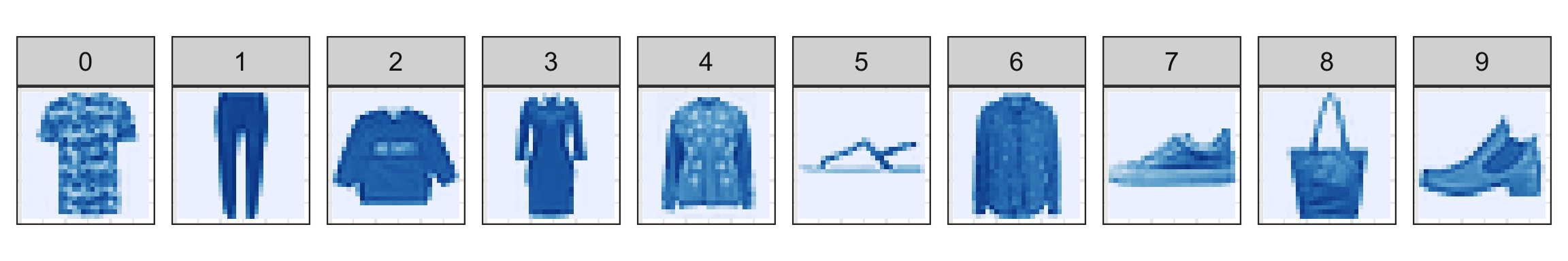
• So this is a multi-class classification problem with m = 10 classes (or levels).
• The training data contains 60,000 observations with 784 variables (pixel1, …, pixel784) and 1 response variable (label) labelled from 0-9.
• The testing data contains 10,000 observations (note: this testing data also contains label!).

Neural network in R 1 prepare the data

• To fit a neural network model, we use the keras package.

• We first need to prepare the data:
  • convert categorical data to dummy variables, and
  • normalise the predictors.

fashion_train_y <- model.matrix(~factor(label) - 1, data = fashion)

fashion_train_x <- fashion %>% 
  select(-label) %>% 
  scale()

fashion_test_y <- model.matrix(~factor(label) - 1, data = fashion_test)

fashion_test_x <- fashion_test %>% 
  select(-label) %>% 
  scale()

Neural network in R 2 Define architechture

library(keras)
NN <- keras_model_sequential() %>% 
  # hidden layer
  layer_dense(units = 128, # number of nodes in hidden layer
              activation = "relu",
              # number of predictors
              input_shape = 784) %>% 
  # output layer
  layer_dense(units = 10, # the number of classes
              # we need to use softmax for multi-class classification
              activation = "softmax")

NN

Model: "sequential"
________________________________________________________________________________
 Layer (type)                       Output Shape                    Param #     
================================================================================
 dense_1 (Dense)                    (None, 128)                     100480      
 dense (Dense)                      (None, 10)                      1290        
================================================================================
Total params: 101,770
Trainable params: 101,770
Non-trainable params: 0
________________________________________________________________________________

Neural network in R 3 Choose loss function

• For regression, you can use mean_squared_error.
• For binary classification, you can use binary_crossentropy.
• For multi-class classfication, you can use categorical_crossentropy.
• For the full list of loss functions, see help("loss-functions").

NNl <- NN %>% 
  compile(loss = "categorical_crossentropy",
          metrics = "accuracy")

Neural network in R 4 Fit model

This model takes long to fit!

learnNNl <- NNl %>% 
  fit(x = fashion_train_x,
      y = fashion_train_y,
      epochs = 20,
      batch_size = 40,
      validation_split = 0.2)

• Typically epochs is a large number.

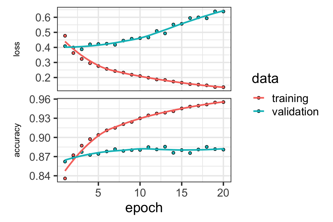
Model diagnostic

• We can plot the loss (and other metrics specified) of the neural network using the plot function on the training history.

class(learnNNl)

[1] "keras_training_history"

plot(learnNNl)

• This model actually is not doing well for the validation set!
• This suggests that the model is overfitted.

Predicting from neural network

• Notice we are using NNl and not learnNNl here!

test_predict <- predict(NNl, fashion_test_x)

test_predict[1:3, ]

             [,1]         [,2]         [,3]         [,4]         [,5]
[1,] 9.959991e-01 4.470216e-15 2.498414e-06 1.280446e-06 6.907984e-09
[2,] 2.188681e-21 1.000000e+00 5.769808e-32 9.360376e-28 1.490198e-26
[3,] 6.637161e-03 6.112183e-16 9.681513e-01 3.647272e-13 6.959190e-06
             [,6]         [,7]         [,8]         [,9]        [,10]
[1,] 2.304835e-11 3.900097e-03 9.305310e-19 9.703544e-05 4.587546e-13
[2,] 0.000000e+00 8.628763e-31 0.000000e+00 4.123140e-29 1.746240e-37
[3,] 8.466854e-11 2.520457e-02 8.891557e-21 6.381754e-13 2.705846e-17

• Each row corresponds to the observation in the test data.
• Column c corresponds to the probability of the label c - 1.
• Sum of each row is 1.

Visually checking the prediction: observation 1

Code

tibble(label = 0:9,
       desc = c("T-shirt/top", "Trouser", "Pullover", "Dress", "Coat", "Sandal", "Shirt", "Sneaker", "Bag", "Ankle boot")) %>% 
  mutate(prob = test_predict[1, ]) %>% 
  ggplot(aes(prob, desc)) +
  geom_col() +
  labs(y = "", x= "Probability")

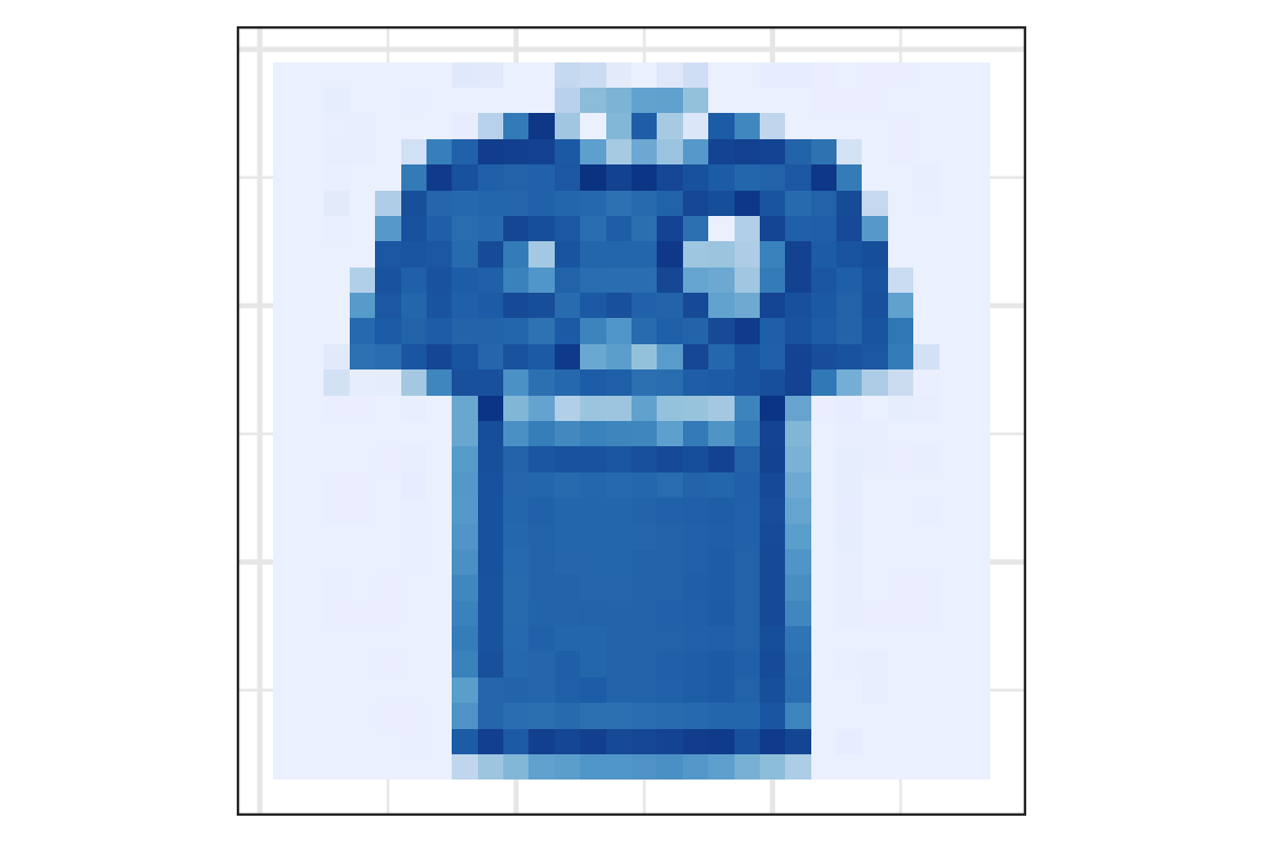
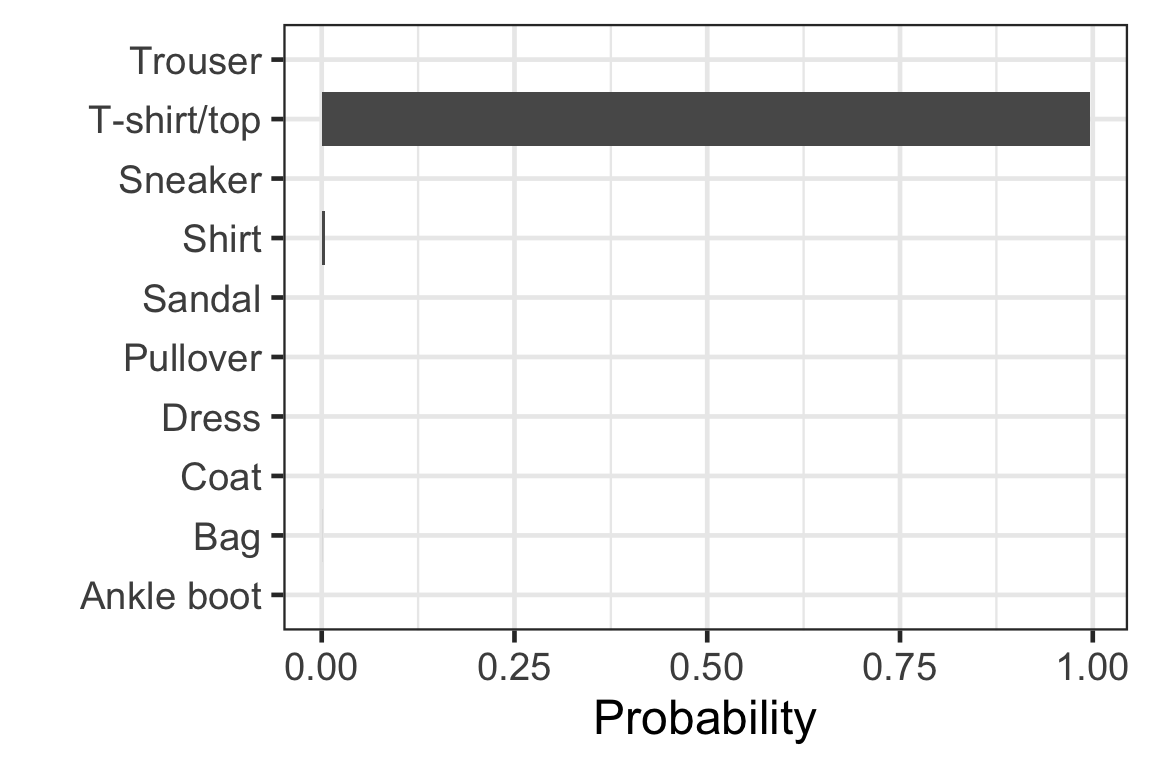
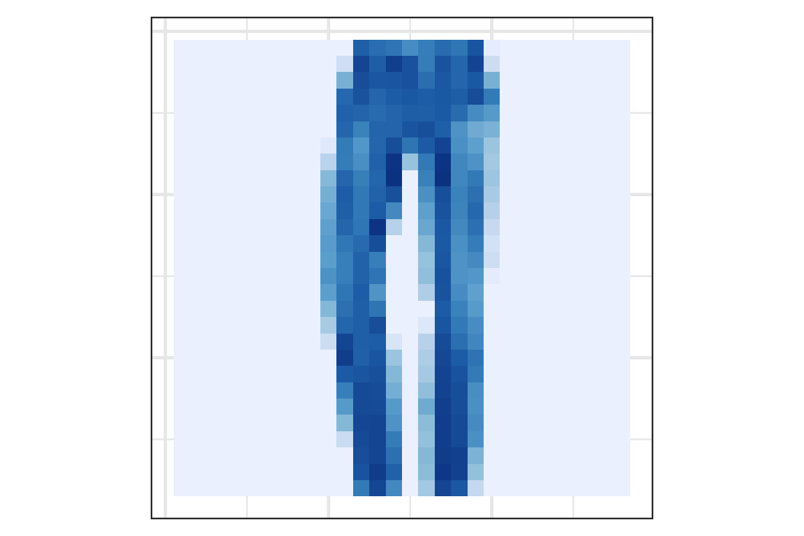
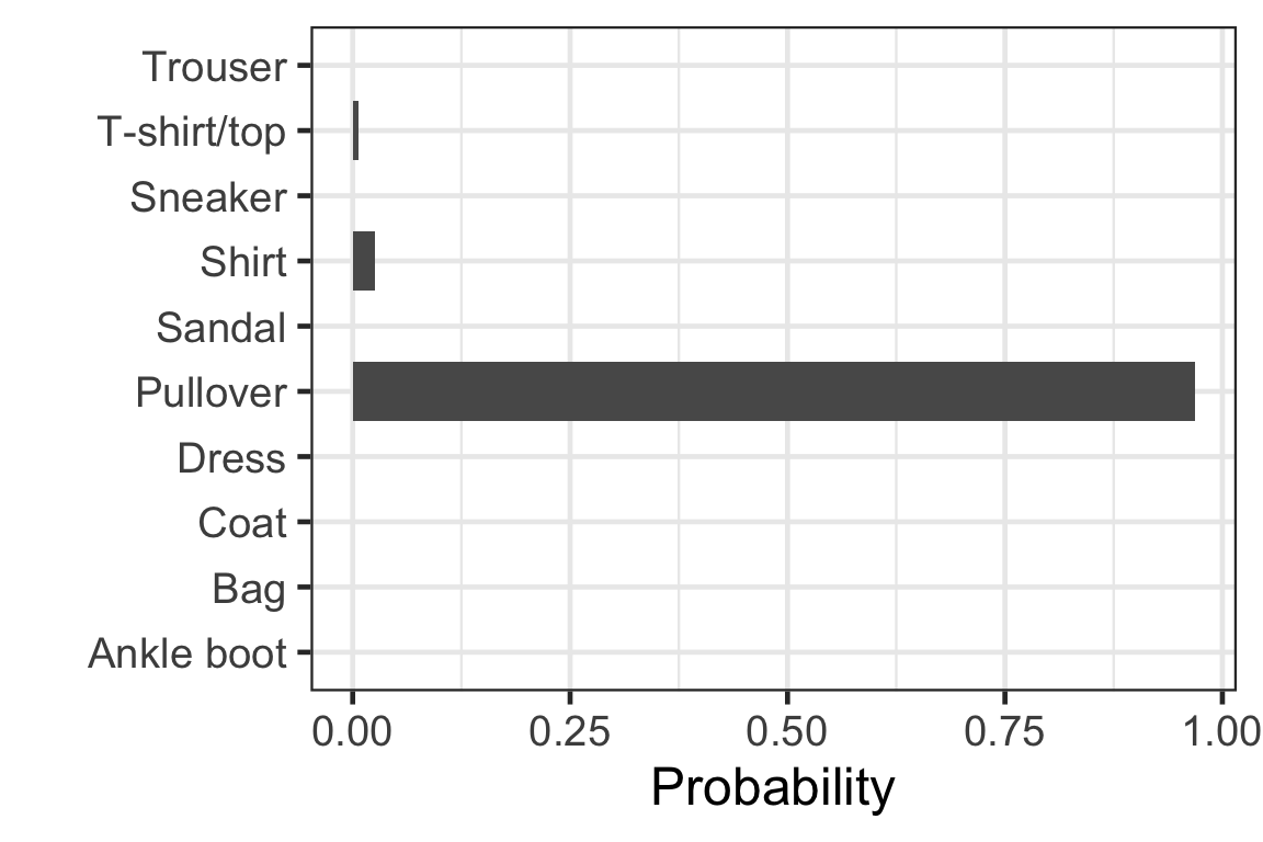
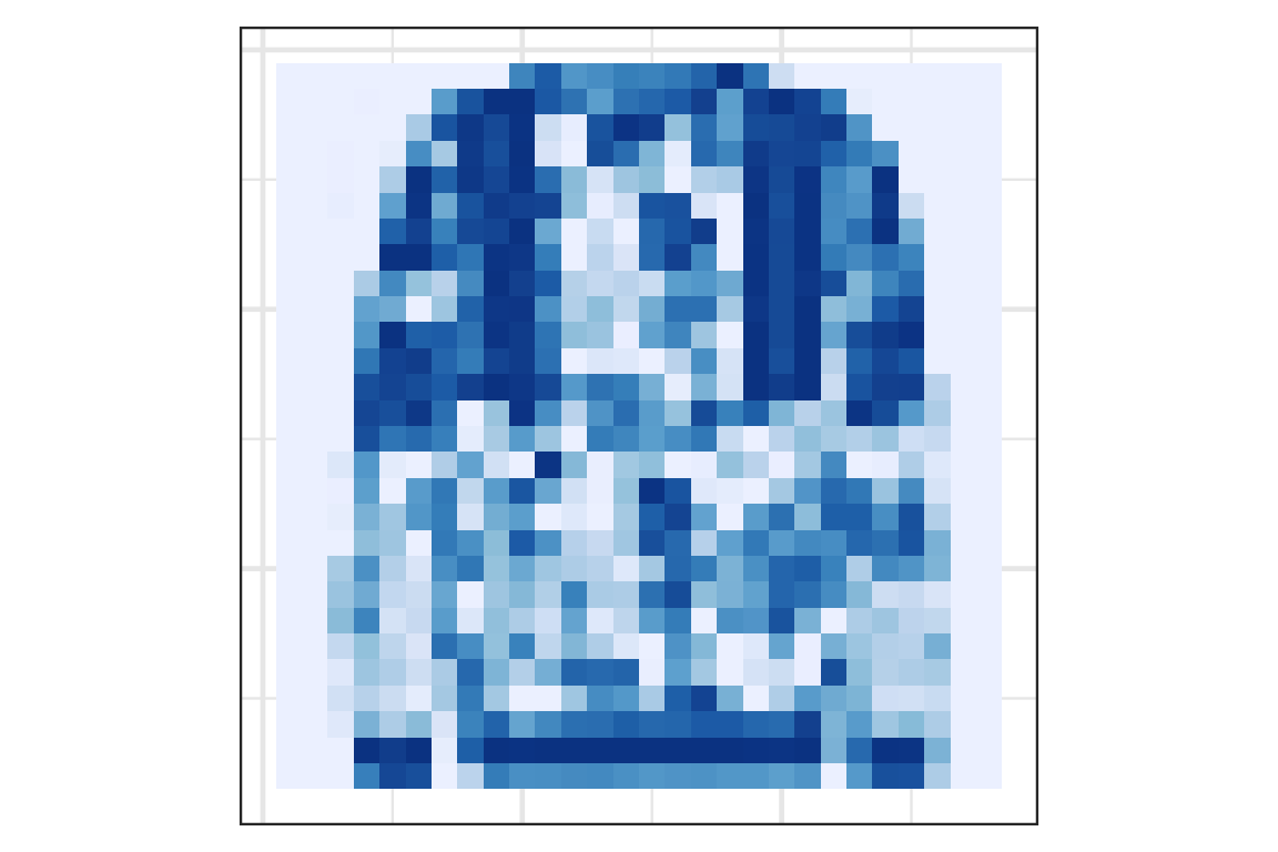
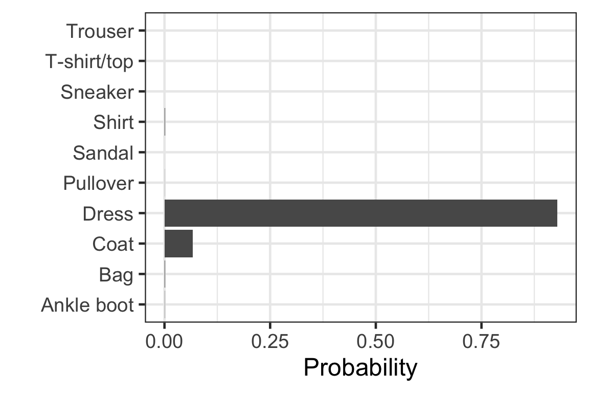
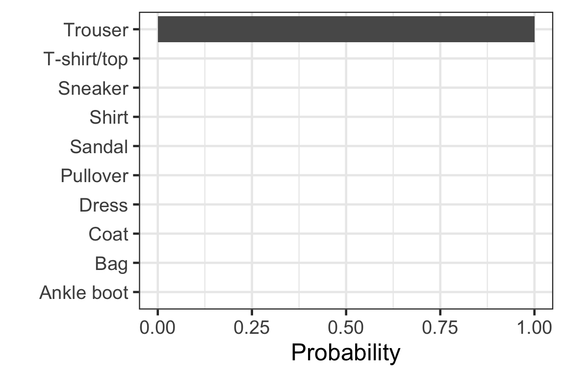
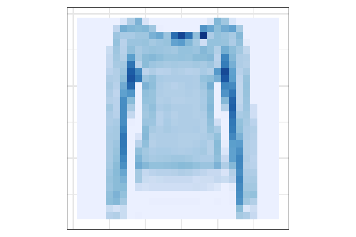
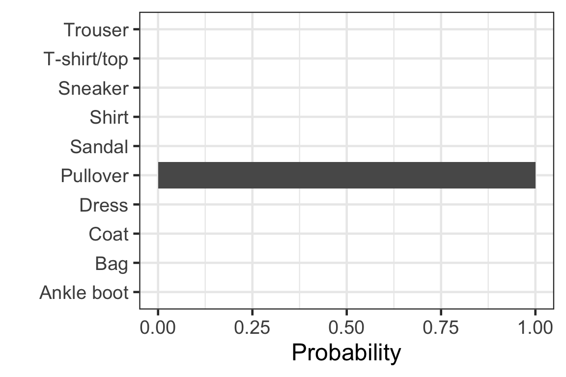
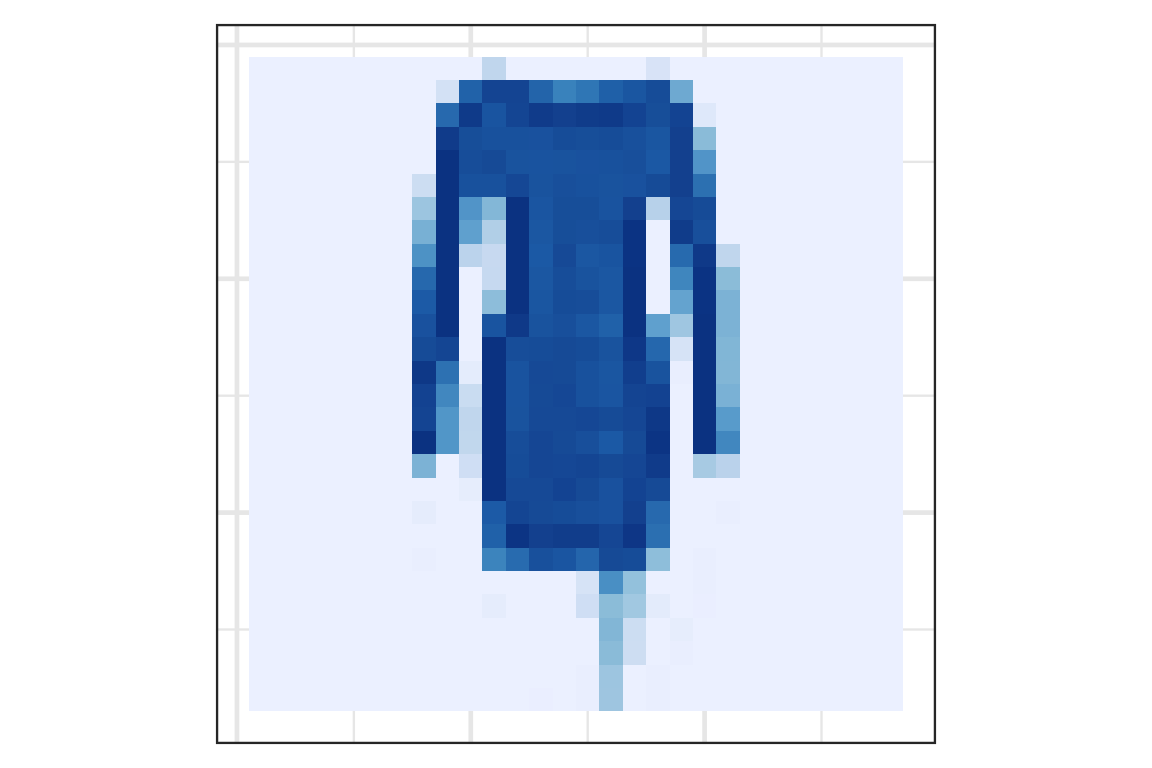
Visually checking the prediction: observation 2

Code

tibble(label = 0:9,
       desc = c("T-shirt/top", "Trouser", "Pullover", "Dress", "Coat", "Sandal", "Shirt", "Sneaker", "Bag", "Ankle boot")) %>% 
  mutate(prob = test_predict[2, ]) %>% 
  ggplot(aes(prob, desc)) +
  geom_col() +
  labs(y = "", x= "Probability")

Visually checking the prediction: observation 3

Code

tibble(label = 0:9,
       desc = c("T-shirt/top", "Trouser", "Pullover", "Dress", "Coat", "Sandal", "Shirt", "Sneaker", "Bag", "Ankle boot")) %>% 
  mutate(prob = test_predict[3, ]) %>% 
  ggplot(aes(prob, desc)) +
  geom_col() +
  labs(y = "", x= "Probability")

Visually checking the prediction: observation 4

Code

tibble(label = 0:9,
       desc = c("T-shirt/top", "Trouser", "Pullover", "Dress", "Coat", "Sandal", "Shirt", "Sneaker", "Bag", "Ankle boot")) %>% 
  mutate(prob = test_predict[4, ]) %>% 
  ggplot(aes(prob, desc)) +
  geom_col() +
  labs(y = "", x= "Probability")

Visually checking the prediction: observation 5

Code

tibble(label = 0:9,
       desc = c("T-shirt/top", "Trouser", "Pullover", "Dress", "Coat", "Sandal", "Shirt", "Sneaker", "Bag", "Ankle boot")) %>% 
  mutate(prob = test_predict[5, ]) %>% 
  ggplot(aes(prob, desc)) +
  geom_col() +
  labs(y = "", x= "Probability")

Limitations

Cons of neural network

• Minimal interpretability.
• Requires the number of observations to be larger than the number of features.
• Computationally intensive
  • Many calculations are required to estimate all of the parameters in many neural networks.
  • Deep learning involves huge amounts of matrix multiplications and other operations.
  • Often used in conjuction with GPUs to parallellise computations.

Takeaways

• To build a feed-forward neural network, we need the key components:
  1. Input data,
  2. A pre-defined network architecture,
  3. A feedback mechanism (e.g. loss function) to enable the network to learn, and
  4. Model training.
• Deep neural networks are faster to calibrate than wide neural networks via stochastic gradient descent and backpropogation algorithms.