ETC3250/5250

Introduction to Machine Learning

Neural network I

Lecturer: Emi Tanaka

Department of Econometrics and Business Statistics

Supervised learning

So far you have learnt about:
- linear, non-linear & logistic regression
- linear & quadratic discriminant analysis
- decision trees
- tree-ensemble methods (bagging, boosting, random forest)
- k-nearest neighbours
- support vector machine methods
But these methods still don’t perform well for some tasks, e.g. image recognition.

Human brain

Our brains can dissect and process features of images, e.g. the shape, object, lighting, etc.

The human brain is made of billions of neurons that communicate via electrochemical signals.

So how do we mimic this in a program?

Artificial neuron

Biological neuron model

Artificial neural network, or often referred to just as neural network, was inspired by the biological neural network.
In a biological neural network, a collection of neurons interconnected by synapses carry out a specific function when activated.

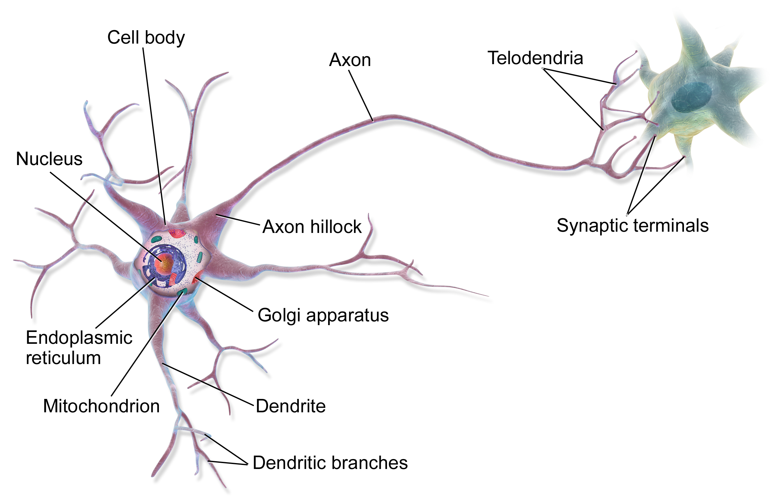
The dendrites receive synaptic inputs and propogate electrochemical stimulation to the cell body - if stimulated enough, a neuron fires an action potential (synaptic inputs for other neurons).

Artificial neuron: dendrites

The artificial neuron is the elementary units of an artificial neural network.

The artificial neuron receives predictors \boldsymbol{x}_i = (1, x_{i1}, \dots,x_{ip})^\top that is typically combined as a weighted sum:

z_i = \beta_0 + \sum_{j=1}^p\beta_jx_{ij} = \boldsymbol{\beta}^\top\boldsymbol{x}_i, \quad\text{where }\boldsymbol{\beta} = (\beta_0, \beta_1, \dots, \beta_p)^\top.

Artificial neuron: action potential

The z_i then get passed into the activation function, h(z_i).
Suppose a is the location parameter and w is the scale parameter.
Some common choices include:
- Heaviside step: h(z_i) = \mathbb{I}(z_i > 0),
- Linear: h(z_i) = z_i,
- Sigmoid: h(z_i|a,w) = a + w(1+e^{-z_i})^{-1},
- Tanh: h(z_i|a,w) = a + w \left(\frac{2}{1+e^{-2z_i}} - 1 \right), and
- ReLU: h(z_i|a,w) = a + w \times \max(0, z_i).

Visualising artifical neuron

When x_1 = 1 and x_2 = 3, then \begin{align*}z &= \beta_0 + \beta_1x_1 + \beta_2 x_2\\ &= 1 + 0.5 \times 1 - 3\times 3 = -7.5.\end{align*}
Using ReLU with a = 1, w = 2, the prediction is 1 + 2 \times \max(0, z) = 1.

Predicting from an artificial neuron

Your turn!

What is the prediction when x_1 = 10?

What is the prediction when x_1 = -5?

-11

Activation function

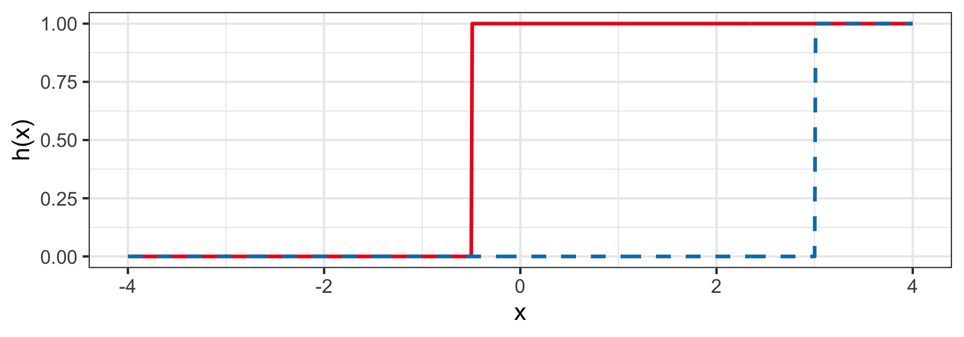
Heaviside step

h(z_i) = \mathbb{I}(z_i > 0)

This is also known as the perceptron and is used for classification.

For example: h(1 + 2x_i) and h(-12 + 4x_i).

Linear

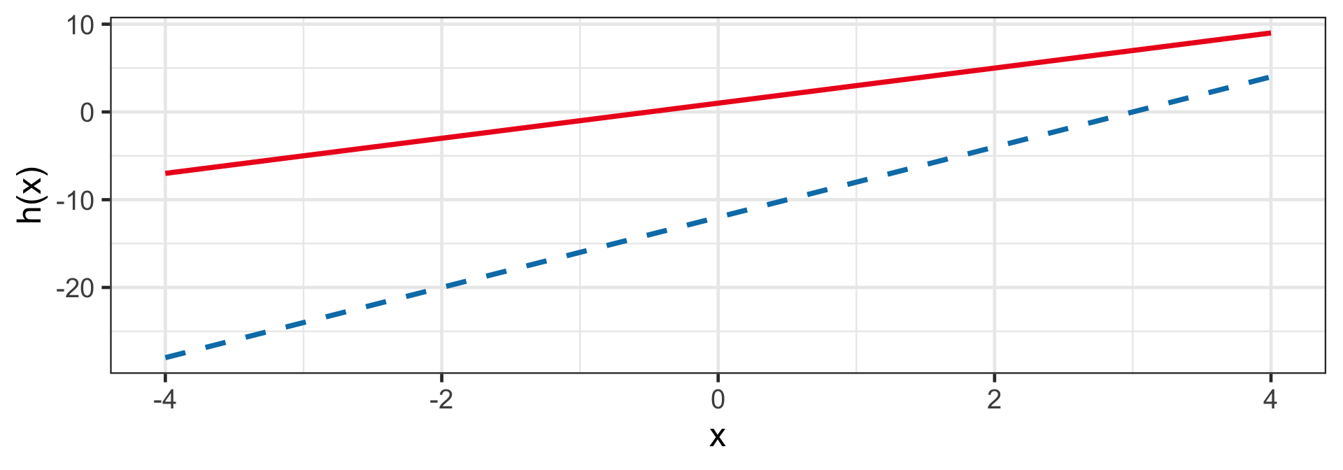
h(z_i) = z_i

This is a regression model!
For example: h(1 + 2x_i) and h(-12 + 4x_i).

Sigmoid (Logistic)

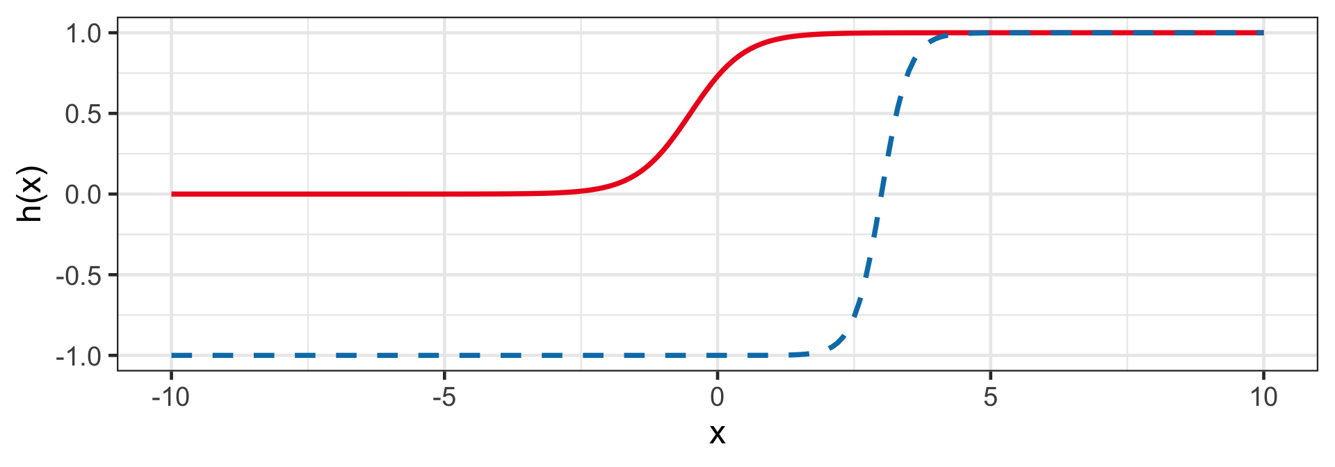
h(z_i|a,w) = a + w(1+e^{-z_i})^{-1}

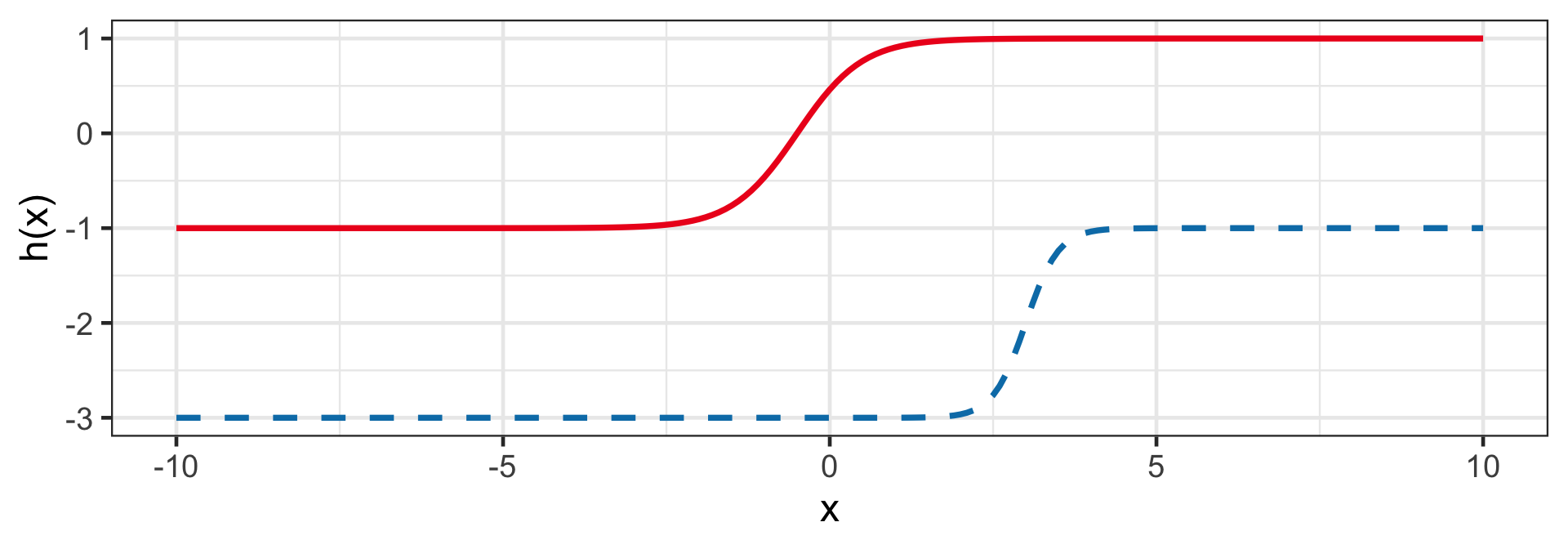
When a = 0 and w = 1, then 0 < h(z_i) < 1 for finite z_i.
E.g. h(1 + 2x_i|a = 0, w = 1) and h(-12 + 4x_i|a = -1, w = 2).

Hyperbolic tangent (Tanh)

h(z_i) = a + w \left(\frac{2}{1+e^{-2z_i}} - 1 \right)

Similar to Sigmoid.
E.g. h(1 + 2x_i|a = 0, w = 1) and h(-12 + 4x_i|a = -1, w = 2).

Rectified linear unit (ReLU)

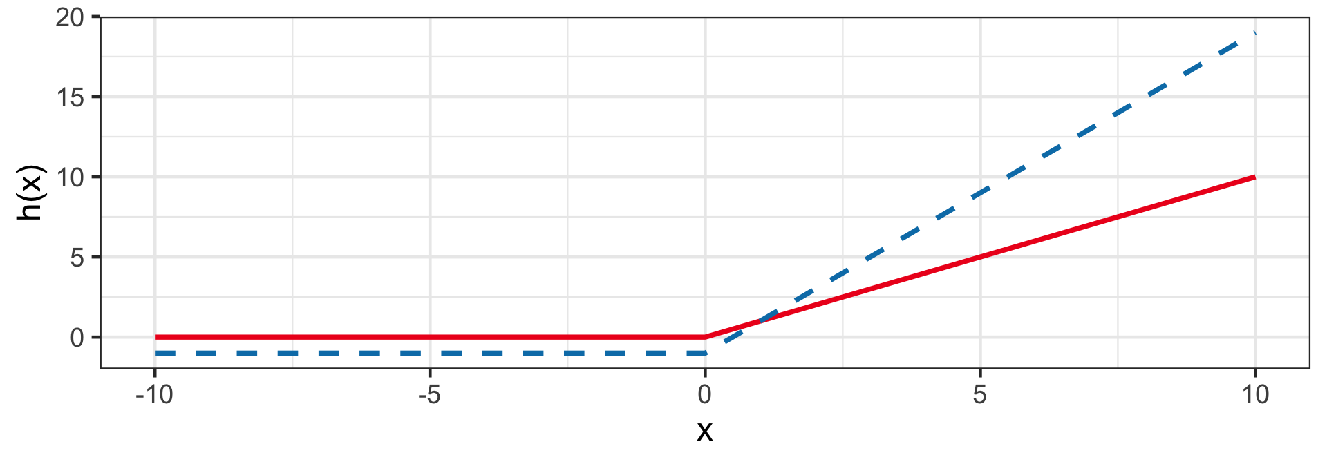
h(z_i) = a + w \times \max(0, z_i)

Sigmoid and Tanh are largely replaced by rectified linear unit (ReLU).
E.g. h(1 + 2x_i|a = 0, w = 1) and h(-12 + 4x_i|a = -1, w = 2).

Neural network

Limitations of a single artificial neuron

Biological neurons are interconnected in complex networks that allow the brain to perform a wide range of functions.
A single artificial neuron has a limited ability to model complex relationships so much like its biological counterpart, we can connect different artificial neurons to model complex relationships.
An artifical neural network, the interconnection of the artificial neurons, began by mimicing the architecture of brain activity.
But neural network is no longer true to their biological counterpart and its development is motivated by empirical results.

Multiple artificial neurons

When combining artificial neurons, we always set a = 0 and w = 1 for Sigmoid, Tanh, and ReLU.

Artificial neuron 1

Artificial neuron 2

Combining artificial neurons for regression

In general, we combine K neurons as f(\boldsymbol{x}_i) = b + \sum_{k=1}^Kw_kh(\boldsymbol{\beta}_k^\top\boldsymbol{x}_i)
- \boldsymbol{\beta}_k is the coefficient of predictors in the k-th artificial neuron,
- b is called the bias,
- w_k is the weight corresponding to the k-th neuron.
The activation function h is always of the same type.

Example of combining artificial neurons

f(\boldsymbol{x}_i) = b + w_1{\color{#027EB6}{h(\boldsymbol{\beta}_1^\top\boldsymbol{x}_i)}} + w_2\color{#EE0220}{h(\boldsymbol{\beta}_2^\top\boldsymbol{x}_i)}

This represents a neural network with

2 nodes in the input layer,
2 nodes in the middle layer, and
1 node in the output layer with parameters:
- b = 0,
- w_1 = 0.5,
- w_2 = 0.9,
- \boldsymbol{\beta}_1 = (3, -5)^\top,
- \boldsymbol{\beta}_2 = (1, 0.5)^\top, and
- h is the ReLU activation function with a = 0 and w = 1.

Combining artificial neurons for classification

The output of the previous example is only applicable for regression problems.
We can easily modify this for classfication by changing the output layers to say the Sigmoid function, which gives a numerical value between 0 and 1 and can be thought of as the propensity score. P(y_i = 1 | \boldsymbol{x}_i) = \frac{1}{1 + \exp\left(-(b + \sum_{k=1}^Kw_kh(\boldsymbol{\beta}_k^\top\boldsymbol{x}_i))\right)}.

Regression vs classification

In a neural network, initial layers can be identical for regression or classification.

It is the output layer that determines if it can be used for regression or classification!

Multi-class classification

The Sigmoid functions allows for computation of propensity scores for binary outcomes.
If you have more than two classes in your response, then you need to convert it to dummy variables, or otherwise referred to as one-hot encoding.
So for a categorical variable with m levels, y_i \in \{\text{Class 1}, \dots, \text{Class }m\}, we convert it as: y_{ik} = \begin{cases}1 & \text{if } y_i = \text{Class}k\\0 & \text{if } y_i \neq \text{Class}k\end{cases}

From categorical variable to dummy variables

dat <- tibble(pet = c("cat", "dog", "cat", "fish"))
model.matrix(~ pet - 1, data = dat)

  petcat petdog petfish
1      1      0       0
2      0      1       0
3      1      0       0
4      0      0       1
attr(,"assign")
[1] 1 1 1
attr(,"contrasts")
attr(,"contrasts")$pet
[1] "contr.treatment"

Alternatively,

class_levels <- as.numeric(factor(dat$pet)) - 1 # changes to cat = 0, dog = 1, fish = 2 
keras::to_categorical(class_levels, num_classes = 3)

     [,1] [,2] [,3]
[1,]    1    0    0
[2,]    0    1    0
[3,]    1    0    0
[4,]    0    0    1

Softmax activation function

The Sigmoid function only works for m = 2.
For m > 2, we can use the Softmax activation function instead: P(y_{ij} = 1 | \boldsymbol{x}_i) = \frac{\exp(\boldsymbol{\beta}_j^\top\boldsymbol{x}_i)}{\sum_{j=1}^m\exp\left(\boldsymbol{\beta}_j^\top\boldsymbol{x}_i\right)}.
The number of neurons for the Softmax layer must be m.
Note that \sum_{j=1}^m P(y_{ij} = 1 | \boldsymbol{x}_i) = 1.

An illustration of a Softmax layer

Suppose we have the income of a customer in thousands of dollar.
We want to predict if the customer will buy a “cheap”, “average” or “expensive” brand of clothing brand.
What is the probability that customer with an income of $45K will buy a cheap brand based on this trained neural network?

Solution

Layer 2

ReLU: \max(0, 49.62 - 0.37 \times 45) = 32.97
ReLU: \max(0, 27.62 - 0.19 \times 45) = 19.07
ReLU: \max(0, -1.72 + 0.35 \times 45) = 14.03

Output layer

Cheap: \frac{\exp(32.97)}{\exp(32.97) + \exp(19.07) + \exp(14.03)} = 0.9999991
Average: \frac{\exp(19.07)}{\exp(32.97) + \exp(19.07) + \exp(14.03)} = 0.00000092
Expensive: \frac{\exp(14.03)}{\exp(32.97) + \exp(19.07) + \exp(14.03)} = 0.0000000059

Prediction: The customer will buy the cheap brand.

Building a neural network structure with R

Installing keras

Keras is an open-source software library that uses the TensorFlow library to fit artificial neural networks.
We can use the Keras library through the keras package in R.
To install keras, run the following commands:

install.packages("keras")
library(keras)
install_keras(method = c("conda"), 
              conda = "auto", 
              tensorflow = "default",
              extra_packages = "tensorflow-hub")

Be warned that the installation poses issues often due to keras looking at the wrong location for the Keras library.

Building a neural network structure in R

library(keras)
model <- keras_model_sequential() %>%
  layer_dense(units = 3,
              input_shape = 2,
              activation = "relu") %>% 
  layer_dense(units = 3, 
              activation = "softmax")

keras_model_sequential() must be used first to initialise the architechture.
layer_dense() indicates a new layer with:
- units indicating the number of neurons in that layer,
- input_shape indicating the number of predictors (only needed for the first layer_dense()),
- activation specifying the activation function for that layer.

Examining the weights and biases

You can extract the weights and biases using get_weights():

get_weights(model)

[[1]]
           [,1]       [,2]       [,3]
[1,]  0.4419321 -0.3501425 -0.0361855
[2,] -0.9320850 -0.9673537  0.7750421

[[2]]
[1] 0 0 0

[[3]]
          [,1]       [,2]      [,3]
[1,] 0.8876681 -0.5565016 0.4099801
[2,] 0.8715661  0.2542915 0.3897784
[3,] 0.9583607  0.3416290 0.6392198

[[4]]
[1] 0 0 0

Every even entry is the bias of the nodes (here all 0s).
The weights are given in every odd entry in the order of the layers.

Manually setting the weights

w <- get_weights(model)
w[[1]] <- matrix(c(49.62, -0.37, 27.62, -0.19, -1.72, 0.35), nrow = 2)
w[[3]] <- diag(3)
set_weights(model, w)
get_weights(model)

[[1]]
      [,1]  [,2]  [,3]
[1,] 49.62 27.62 -1.72
[2,] -0.37 -0.19  0.35

[[2]]
[1] 0 0 0

[[3]]
     [,1] [,2] [,3]
[1,]    1    0    0
[2,]    0    1    0
[3,]    0    0    1

[[4]]
[1] 0 0 0

Let’s manually set the weights as the previous example:

Prediction from neural network model

Normally we need to train the model but this will be covered next week.
Suppose the manually set weights are a result from a trained model.

You can predict the probability a customer with an income of $45K will buy a cheap, average or expensive brand with:

predict(model, cbind(1, 45))

         [,1]        [,2]         [,3]
[1,] 0.999999 9.18979e-07 5.949233e-09

Note that you need to have the new data in a matrix format with the intercept!

Takeaways

Neural networks are flexible models that can be used for both regression and classification problems.
The activation function in the output layer determine if the neural network can be used for regression or classification.
More neural network to come next week!