Department of Econometrics and Business Statistics
Hyperplane
In a p-dimensional space, a hyperplane is a linear subspace of dimension p - 1.
A p-dimensional hyperplane is given as
\beta_0 + \beta_1 x_1 + \dots + \beta_p x_p = 0.
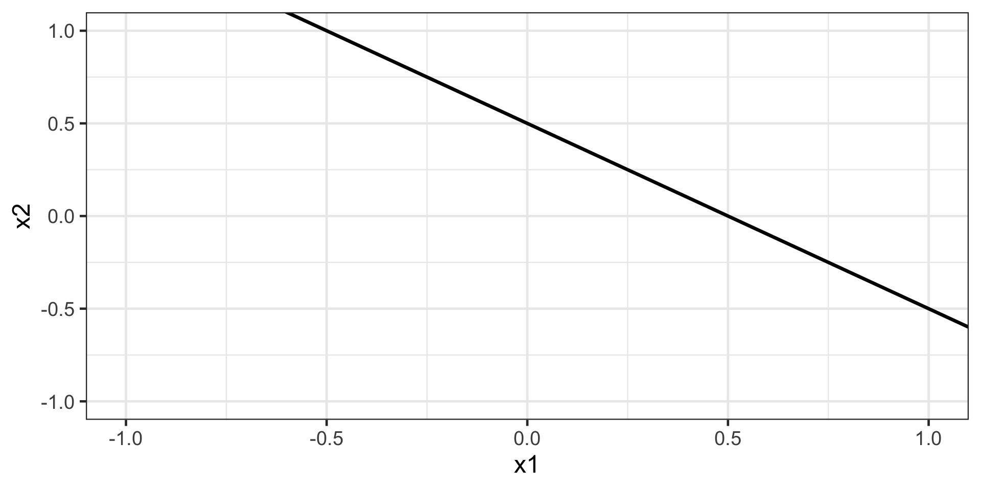
Hyperplane in 2D
For p = 2, a hyperplane is a line.
Hyperplane in 3D
For p = 3, a hyperplane is a plane.
Separating hyperplanes
A hyperplane divides the p-space into two sides.
Suppose we have a new observation \boldsymbol{x}_0 = (x_{01}, x_{02}, \dots, x_{0p})^\top with g(x_0) = \beta_0 + \beta_1 x_{01} + \dots + \beta_p x_{0p}.
\boldsymbol{x}_0 is on side 1 if g(\boldsymbol{x}_0) > 0.
\boldsymbol{x}_0 is on side 2 if g(\boldsymbol{x}_0) < 0.
\boldsymbol{x}_0 is on the hyperplane if g(\boldsymbol{x}_0) = 0.
The magnitude of g(\boldsymbol{x}_0) tells us how far from \boldsymbol{x}_0 is from the hyperplane.
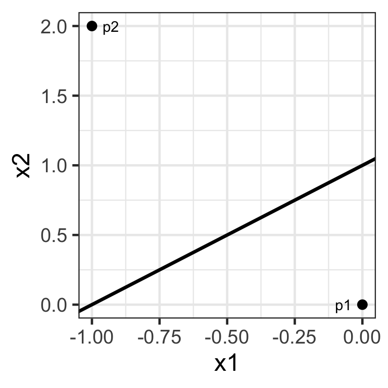
Example
Suppose we have g(\boldsymbol{x}) = 1 + x_{1} - x_2.
Consider the points \boldsymbol{p}_1 = (0, 0)^\top and \boldsymbol{p}_2 = (0, 2)^\top.
\boldsymbol{p}_1 is on side 1.
\boldsymbol{p}_2 is on side 2.
SVM disambiguation
Support vector machine methods refer to three main approaches:
Maximal margin classifier.
Support vector classifier.
Support vector machines.
To avoid confusion, we call these as support vector machine methods and reserve the name support vector machines for the third approach.
Maximal marginal classifier
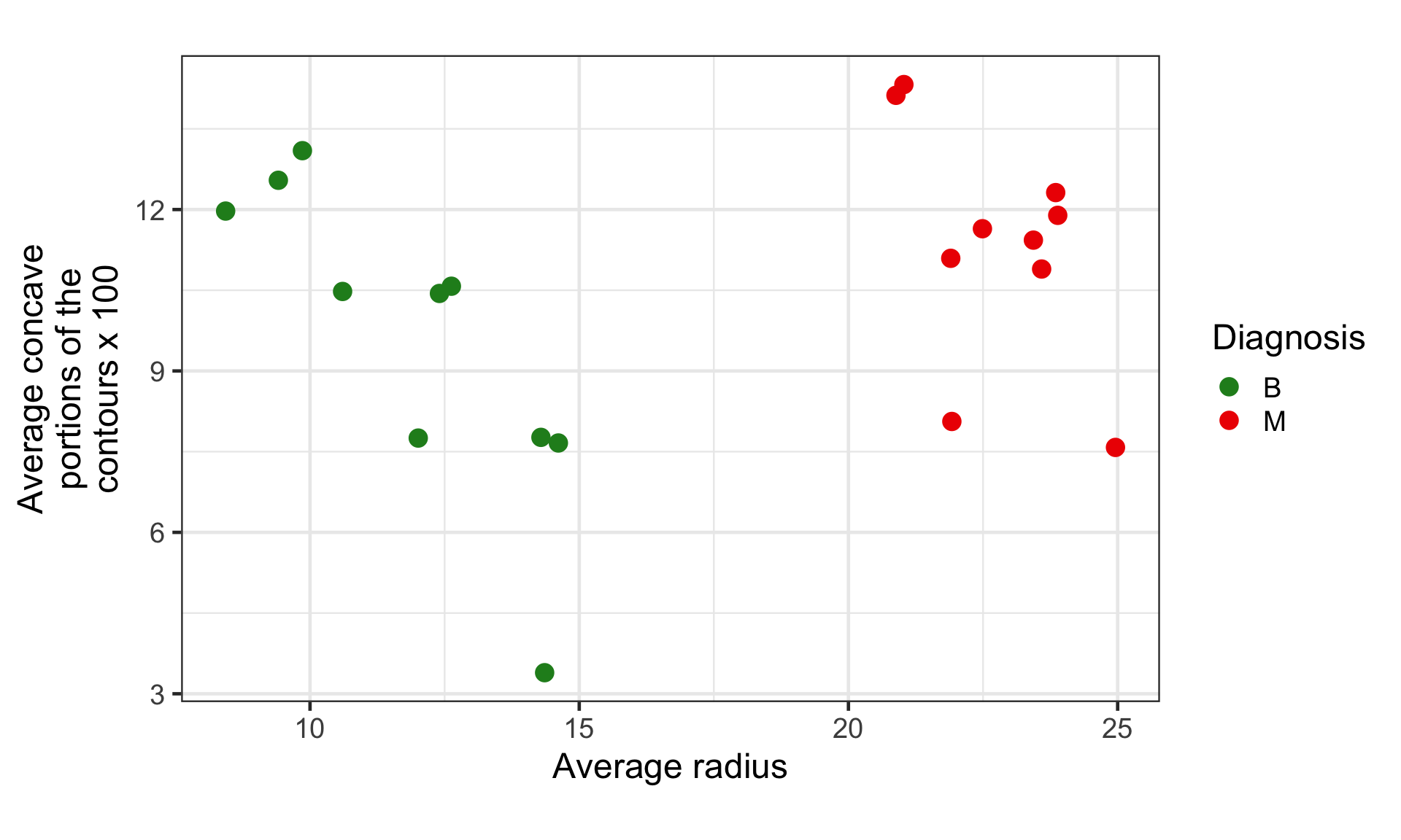
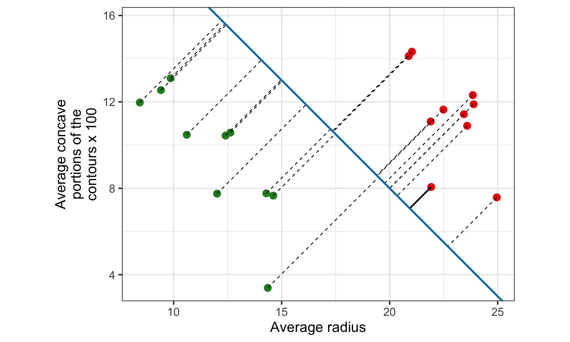
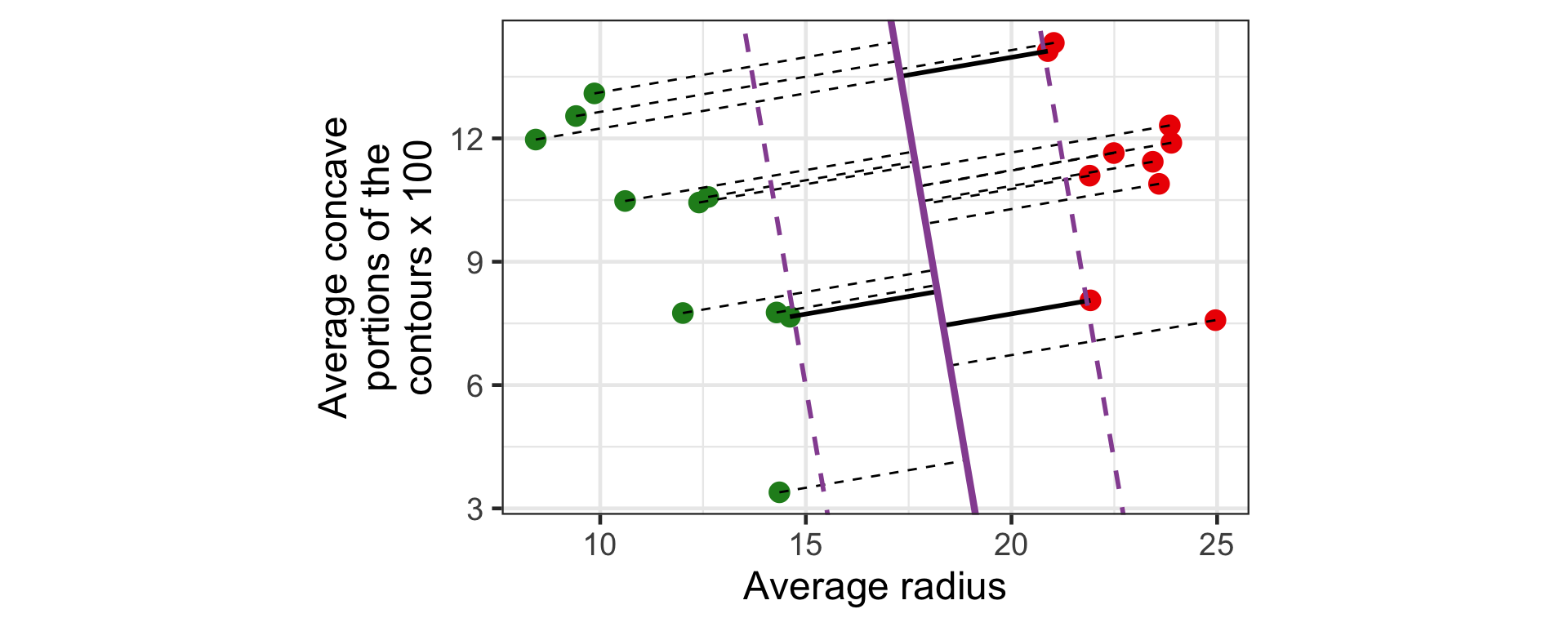
Toy breast cancer diagnosis data
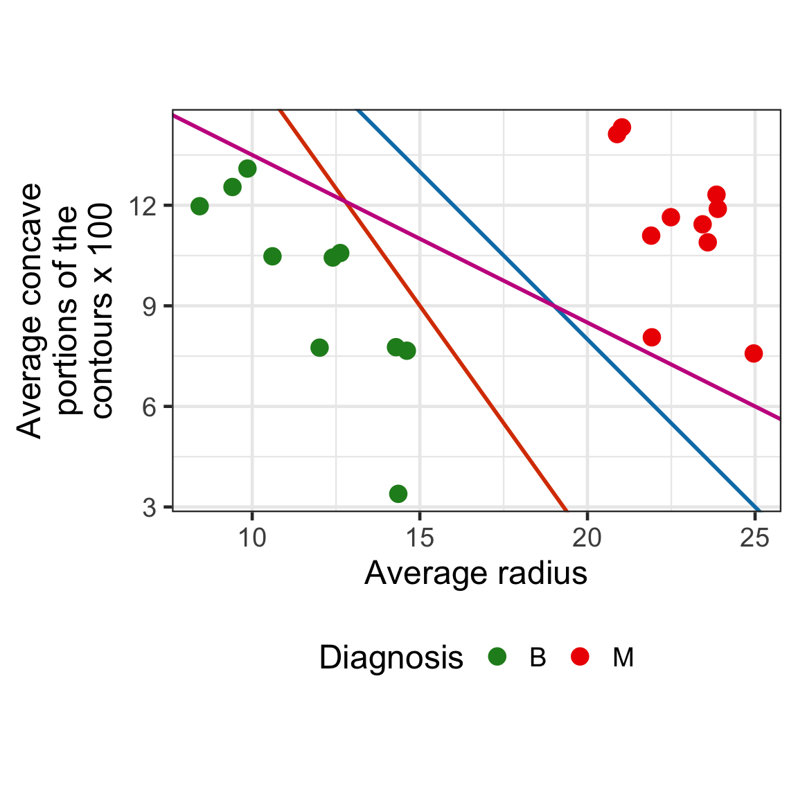
Infinite hyperplanes
There are infinite number of hyperplanes to perfectly classify these points. E.g.,
28 - x_{1} - x_{2} = 0
30 - 1.4x_{1} - x_{2} = 0
18.5 - 0.5x_{1} - x_{2} = 0
All three do a perfect job to separate the classes.
Which one should be we choose?
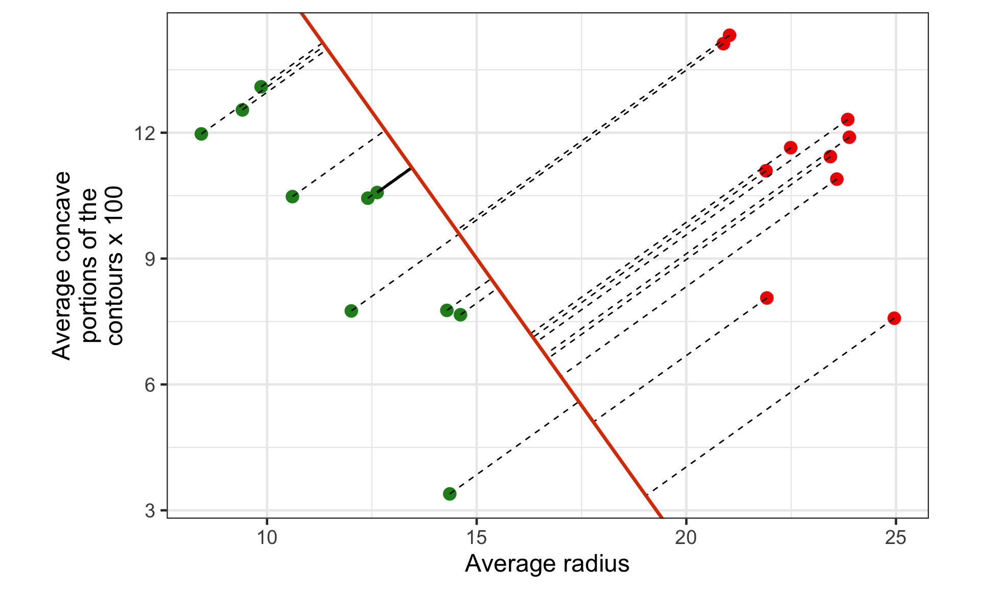
Distance to hyperplane
We compute the (perpendicular) distance from each training observation to a given separating hyperplane.
The smallest such distance is known as the margin (M).
The maximal margin hyperplane is the separating hyperplane for which the margin is largest.
We can then classify a test observation based on which side of the maximal margin hyperplane it lies.
This is known as the maximal margin classifier.
Margin for hyperplane (a)
The margin for this hyperplane is 1.4.
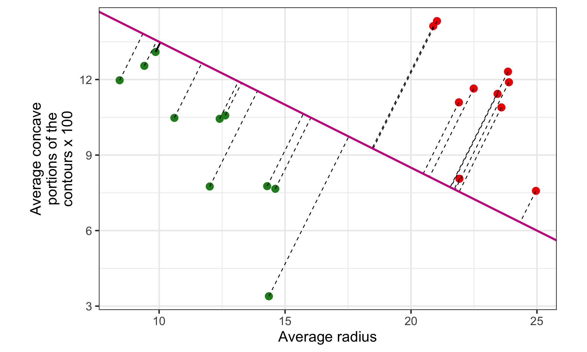
Margin for hyperplane (b)
The margin for this hyperplane is 1.02.
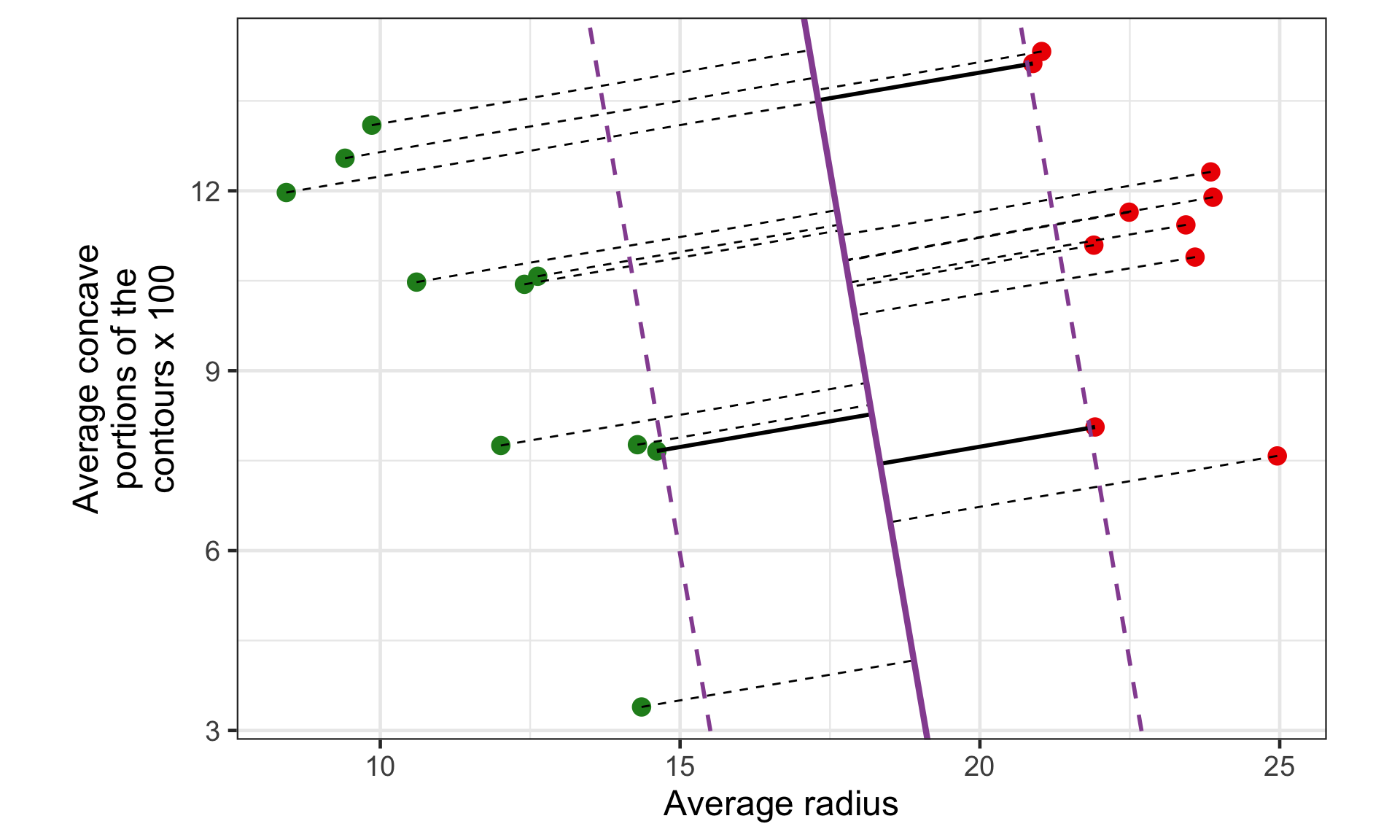
Margin for hyperplane (c)
The margin for this hyperplane is 0.43.
Maximal margin classifier
The maximal margin hyperplane is the plane that correctly classifies all observations but also is farthest away from them.
Support vectors
There will always be at least two equidistant vectors vectors to the maximal margin hyperplane.
These are called support vectors – there are three in this example.
Maximal margin hyperplane
Suppose that y_i = \begin{cases}1 & \text{if observation $i$ in class 1}\\-1& \text{if observation $i$ in class 2}\end{cases}.
The maximal margin hyperplane is found from solving the optimisation problem: \hat{\boldsymbol{\beta}} = \arg\max_{\boldsymbol{\beta}\in\mathbb{R}^{p+1}}M subject to \sum_{j=1}^p \beta_j^2 = 1 and y_i \times g(\boldsymbol{x}_i) \geq M.
Non-separable case
The maximal margin classifier only works when we have perfect separability in our data.
What do we do if data is not perfectly separable by a hyperplane?
The support vector classifier allows points to either lie on the wrong side of the margin, or on the wrong side of the hyperplane altogether.
Support vector classifier
Support vector classifier
Support vector classifier allows some observation to be closer to the hyperplane than the support vectors.
It also allows some observations to be on the incorrect side of the hyperplane (i.e. allows for some misclassification).
It will try to classify the remaining observations to be classified correctly.
Optimisation
For support vector classification, we solve the optimisation problem: \hat{\boldsymbol{\beta}} = \arg\max_{\boldsymbol{\beta}\in\mathbb{R}^{p+1}}M subject to \sum_{j=1}^p \beta_j^2 = 1 and y_i \times g(\boldsymbol{x}_i) \geq M(1 - \varepsilon_i).
\varepsilon_i \geq 0 is called the slack variable and \sum_{i=1}^n\varepsilon_i \leq C.
If 0 < \varepsilon_i \leq 1, observation i is correctly classified but it violates the margin.
If \varepsilon_i > 1, observation is incorrectly classified.
Tuning parameter C
C restricts the magnitude of \varepsilon_i.
If C = 0, then all \varepsilon_i = 0 thus support vector classifier is equivalent to maximum margin classifier.
You can select C using cross-validation.
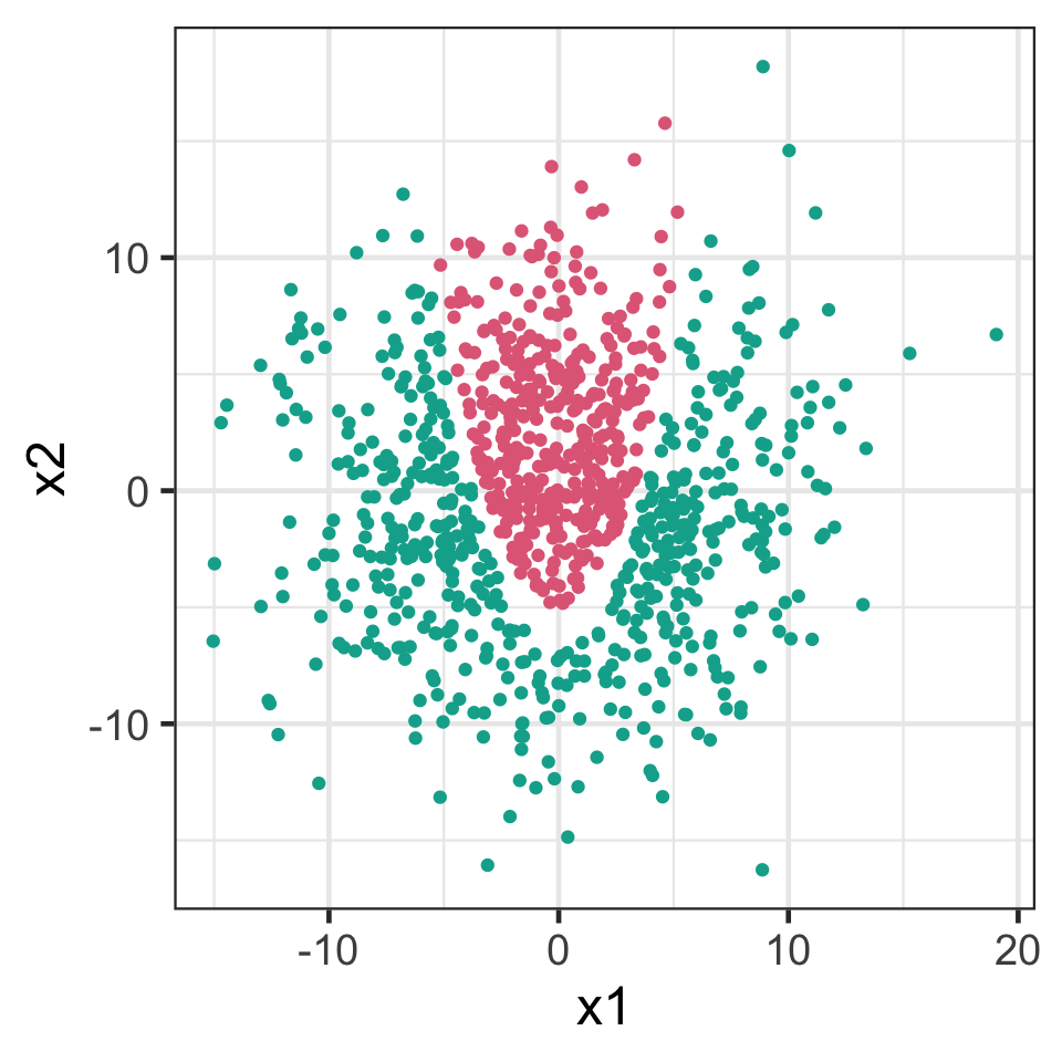
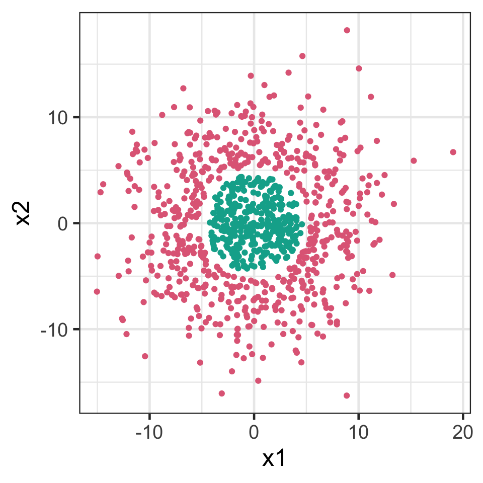
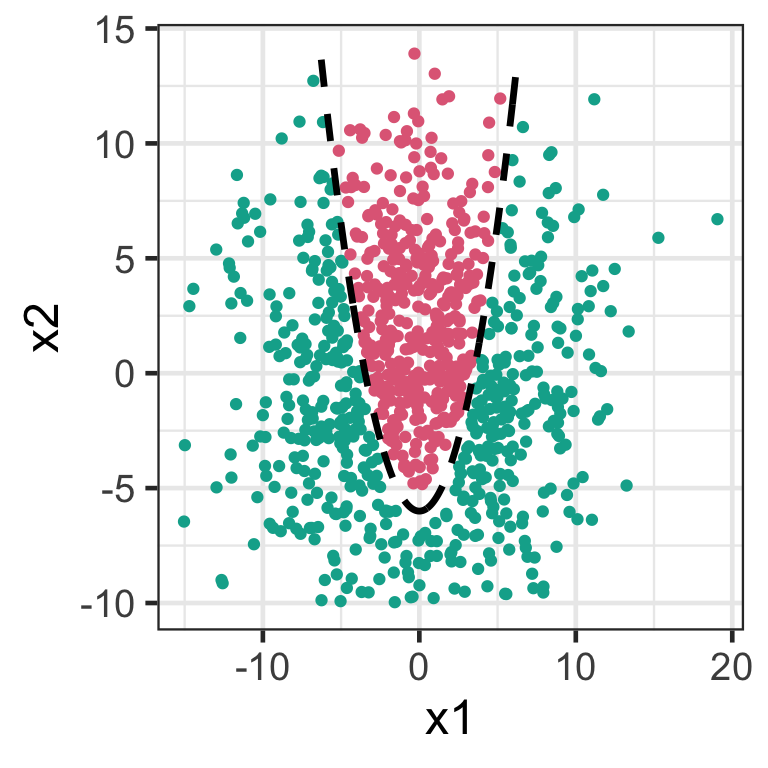
Nonlinear boundaries
The support vector classifier is a linear classifier.
It doesn’t work well for nonlinear boundaries.
Enlarging the feature space
We can make support vector classifier more flexible by adding higher order polynomial terms, e.g. x_1^2 and x_2^3.
We treat these new terms as predictors (referred to as enlarging the feature space).
Support vector machines
Support vector machines
Adding polynomial terms makes support vector classifiers more flexible, but we have to explicitly specify this apriori.
Support vector machines enlarges the feature space without explicit specification of nonlinear terms apriori.
To understand support vector machines, we need to know about:
In support vector machines, we write \beta_j = \sum_{k=1}^n\alpha_ky_kx_{kj}.
This re-expresses g(\boldsymbol{x}) as g(\boldsymbol{x}_i) = \beta_0 + \sum_{j=1}^p\beta_jx_{ij} = \beta_0 + \sum_{k=1}^n\alpha_ky_k\langle\boldsymbol{x}_i, \boldsymbol{x}_k\rangle.
Dual representation
We can generalise the expression by replacing the inner product with a kernel function: g(\boldsymbol{x}_i) = \beta_0 + \sum_{j=1}^p\beta_jx_{ij} = \beta_0 + \sum_{k=1}^n\alpha_ky_k\color{#006DAE}{\mathcal{K}(\boldsymbol{x}_i, \boldsymbol{x}_k)}.
Under this representation, we don’t need to manually enlarge the feature space.
Instead we choose a kernel function.
Kernel functions
A kernel function is an inner product of vectors mapped to a (higher dimensional) feature space
\mathcal{K}(\boldsymbol{x}_i, \boldsymbol{x}_k) = \langle \psi(\boldsymbol{x}_i), \psi(\boldsymbol{x}_j) \rangle
\psi: \mathbb{R}^p \rightarrow \mathbb{R}^d
where d > p.
The optimisation problem in the support vector machine methods is hard to solve for large sample size.
It often fails when class overlap in the feature space is large.
It does not have statistical foundation.
Takeaways
There are three types of support vector machine methods:
Maximal margin classifier is for when the data is perfectly separated by a hyperplane
Support vector classifier/soft margin classifier for when data is not perfectly separated by a hyperplane but still has a linear decision boundary, and
Support vector machines used for when the data has nonlinear decision boundaries.