ETC3250/5250
Introduction to Machine Learning
Clustering
Lecturer: Emi Tanaka
Department of Econometrics and Business Statistics
Cluster analysis
- So far we have been working with cases where we have a response of interest (labelled data).
- In some instances, we only have a set of variables but no response of interest (unlabelled data).
- But we may be interested in finding an unobserved grouping within this unlabelled data, e.g. customer segmentation in marketing analysis.
- This is an example of unsupervised learning.
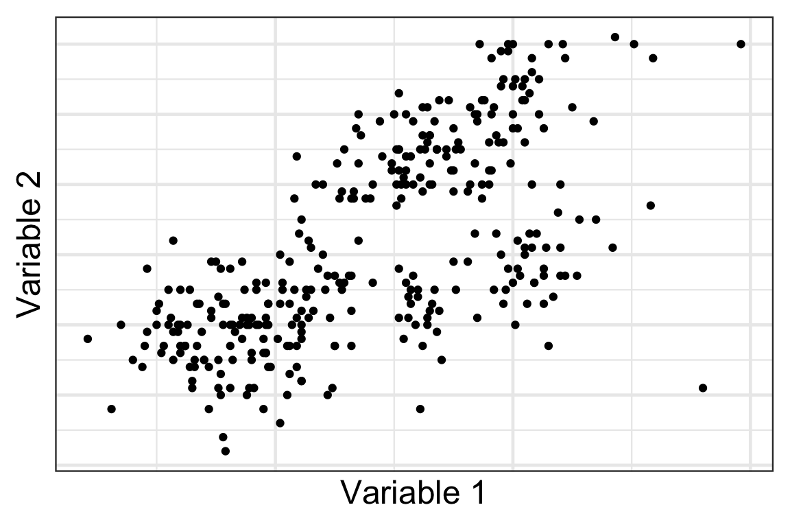
How many clusters do you see?
A possible clustering
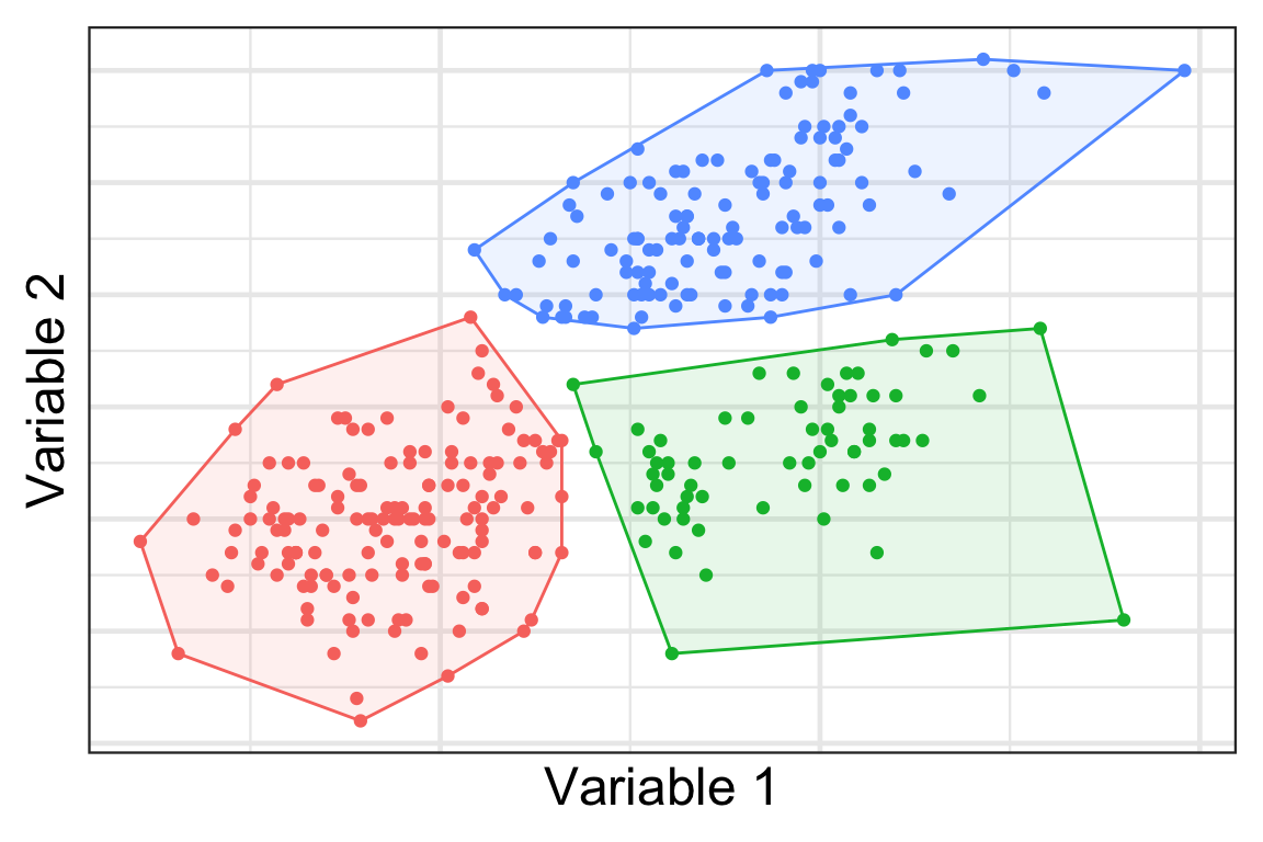
- Here we cluster the observations into 3 groups… but how?
Approaches to clustering
- Hierarchical:
- Agglomerative: One to all.
- Divisive: All to one.
- Non-hierarchical:
- Select the number of clusters.
- Then assign observations to clusters.
- We’ll use k-means clustering to show this.
Hierarchical clustering
Distance
- For clustering, we are grouping observations that are similar.
- Recall from Lecture 7, we covered some distance metrics.
- For clustering, we need two notions of distance:
- Distance between observations
- Distance between clusters
- Let’s denote \mathcal{A} and \mathcal{B} as the two sets that contain the observation indexes of the two clusters, e.g. \mathcal{A} = \{1, 4\} and \mathcal{B} = \{2, 3, 5\} denotes that observations 1 and 4 are in the first cluster and observations 2, 3 and 5 are in the second cluster.
Hierarchical clustering
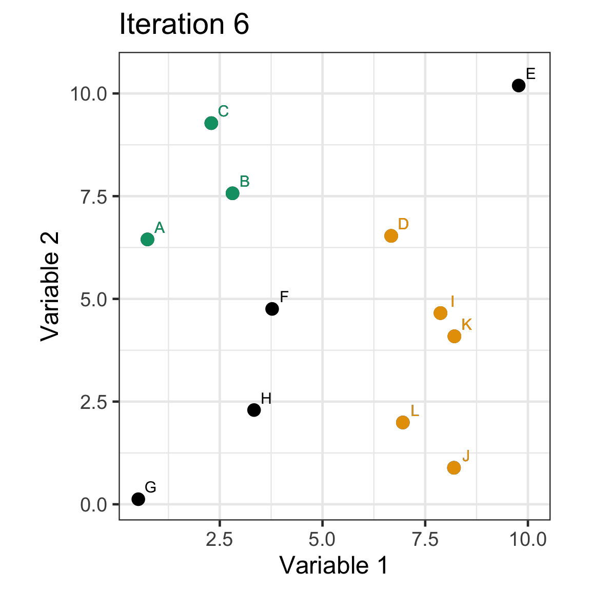
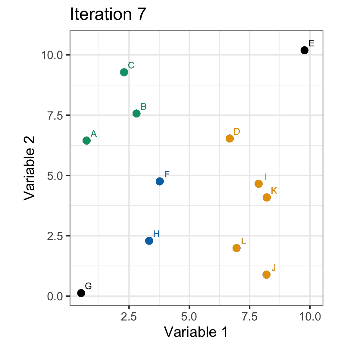
- Agglomerative: Start with all observations in singleton clusters. Merge clusters sequentially until all are in one cluster.
- The functions
hclust()oragnes()can be used for this. - Divisive: Start with all observtions in one cluster, and sequentially divide until all observations are in singleton clusters.
- The function
diana()can be used for this.
Agglomeration method
- There are several ways to merge clusters:
- Single linkage: D(\mathcal{A}, \mathcal{B}) = \min_{i\in\mathcal{A},j\in\mathcal{B}}D(\boldsymbol{x}_i,\boldsymbol{x}_j)
- Complete linkage: D(\mathcal{A}, \mathcal{B}) = \max_{i\in\mathcal{A},j\in\mathcal{B}}D(\boldsymbol{x}_i,\boldsymbol{x}_j)
- Average linkage: D(\mathcal{A}, \mathcal{B}) = \frac{1}{|\mathcal{A}||\mathcal{B}|}\sum_{i\in\mathcal{A}}\sum_{j\in\mathcal{B}}D(\boldsymbol{x}_i,\boldsymbol{x}_j)
- Centroid linkage: D(\mathcal{A}, \mathcal{B}) = D(\bar{\boldsymbol{x}}_\mathcal{A},\bar{\boldsymbol{x}}_\mathcal{B}), combining based on distance between the centroid location of the each cluster
- Ward’s method: minimises the total within-cluster variance by merging clusters with minimum between-cluster distance.
Toy data
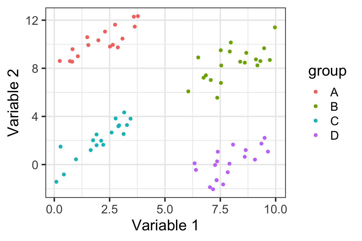
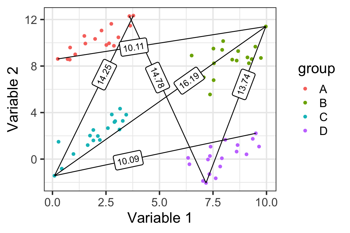
- Suppose we have this data with four groups shown below.
Single linkage
D(\mathcal{A}, \mathcal{B}) = \min_{i\in\mathcal{A},j\in\mathcal{B}}D(\boldsymbol{x}_i,\boldsymbol{x}_j)
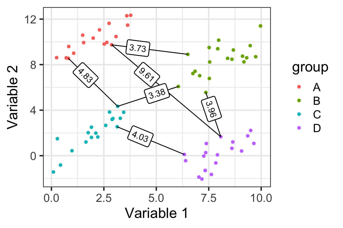
- Here we have 4 groups and 6 distances (based on ED) between clusters.
Complete linkage
D(\mathcal{A}, \mathcal{B}) = \max_{i\in\mathcal{A},j\in\mathcal{B}}D(\boldsymbol{x}_i,\boldsymbol{x}_j)
Average linkage
D(\mathcal{A}, \mathcal{B}) = \frac{1}{|\mathcal{A}||\mathcal{B}|}\sum_{i\in\mathcal{A}}\sum_{j\in\mathcal{B}}D(\boldsymbol{x}_i,\boldsymbol{x}_j)
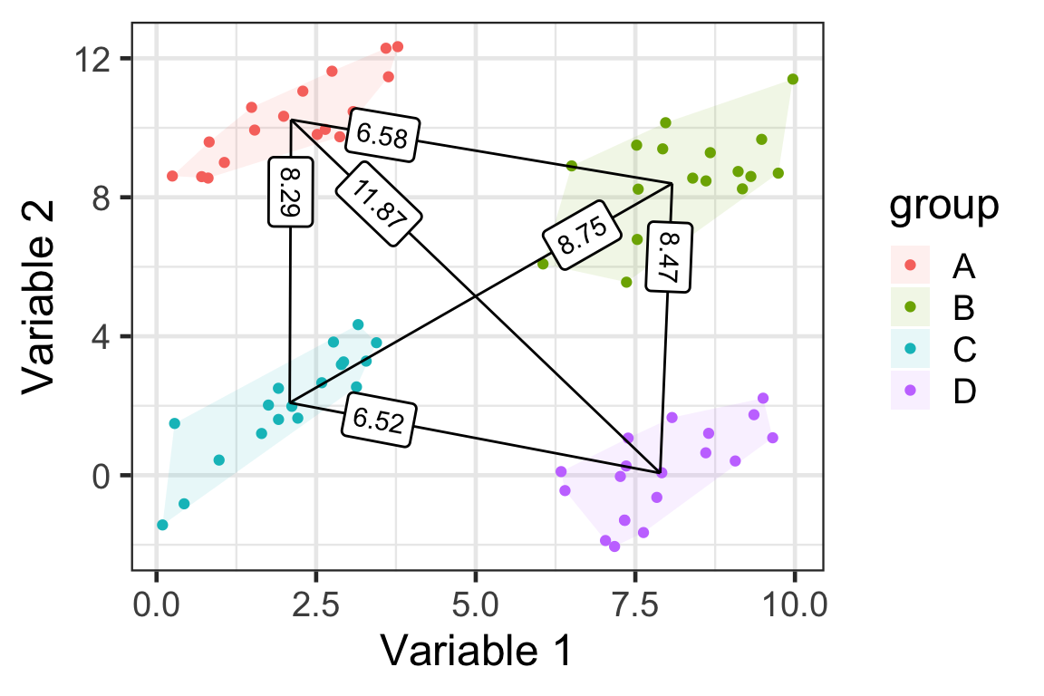
Centroid linkage
D(\mathcal{A}, \mathcal{B}) = D(\bar{\boldsymbol{x}}_\mathcal{A},\bar{\boldsymbol{x}}_\mathcal{B})

Ward’s method
Minimises the total within-cluster sum of squares: W = \sum_{k = 1}^g \left(\sum_{i\in\mathcal{A}_k}\sum_{j=1}^p\left(x_{ij} - \bar{x}_{\cdot j}\right)^2\right) where:
- \bar{x}_{\cdot j} = \frac{1}{|\mathcal{A}_k|}\sum_{i\in\mathcal{A}_k}x_{ij},
- \mathcal{A}_k is a set of indexes for the k-th group,
- g is the number of cluster groups.
Single linkage demo: iteration 0
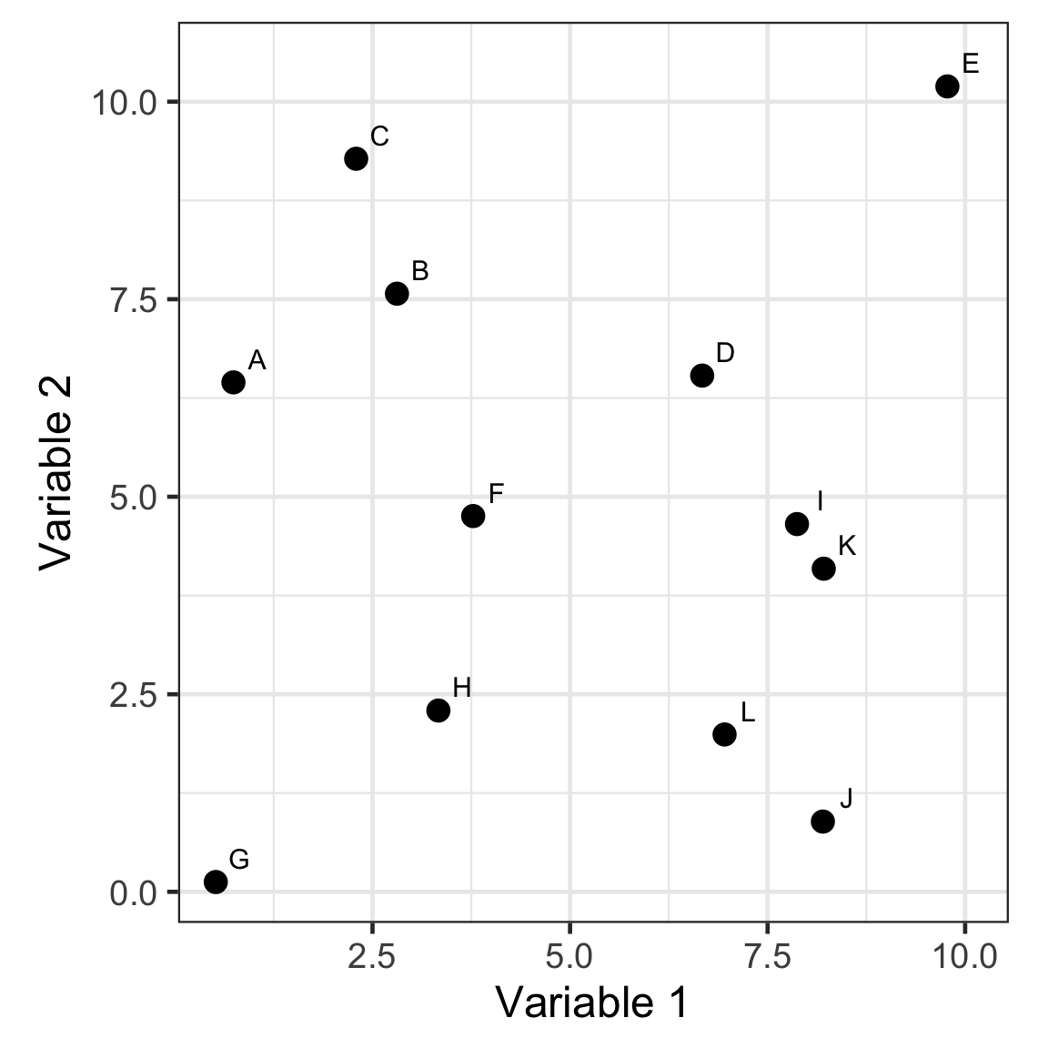
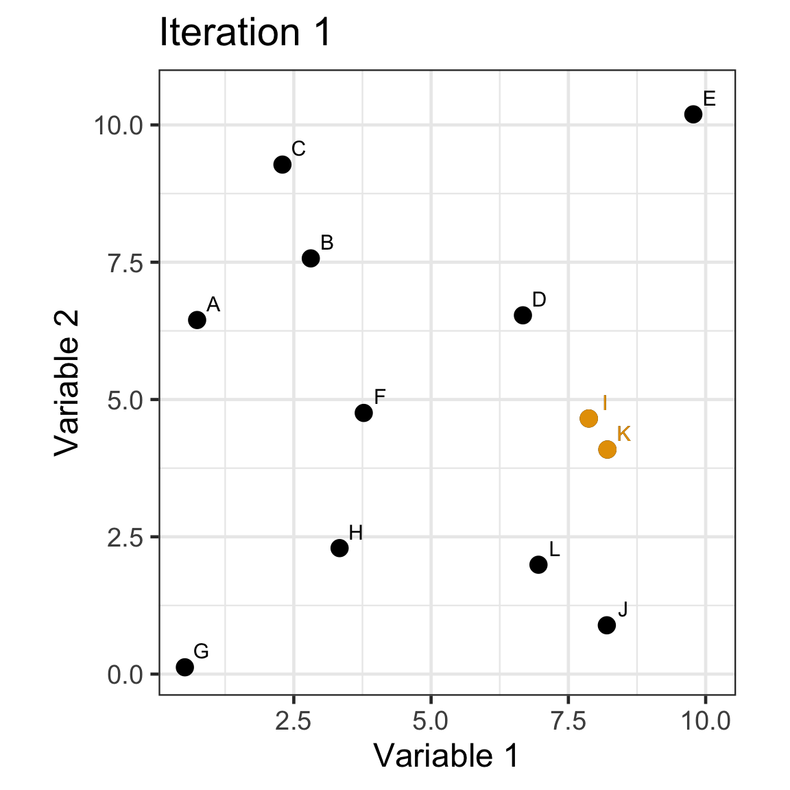
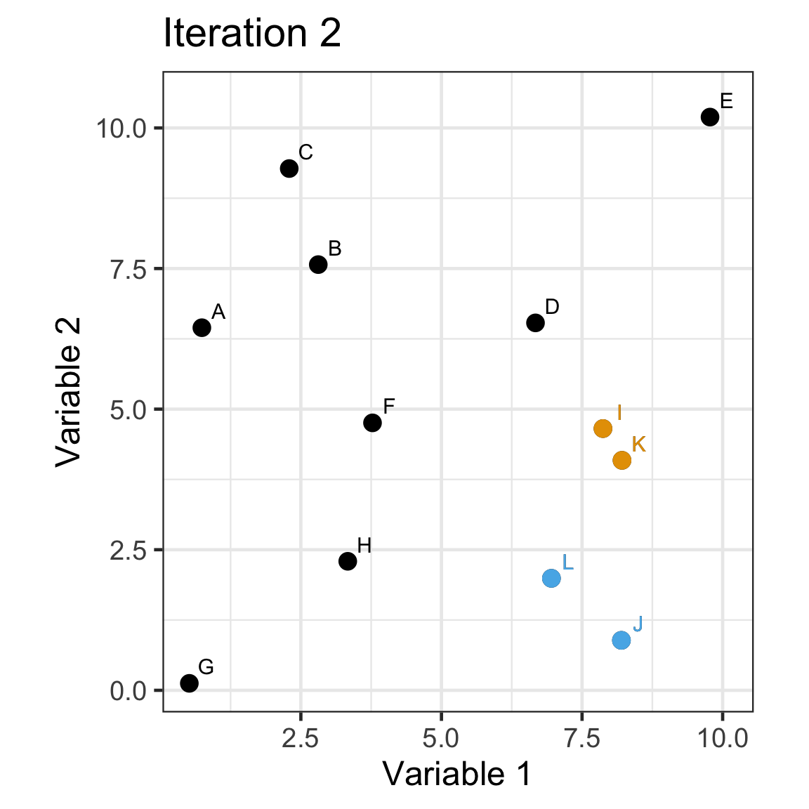
- Every observation starts as a singleton cluster.
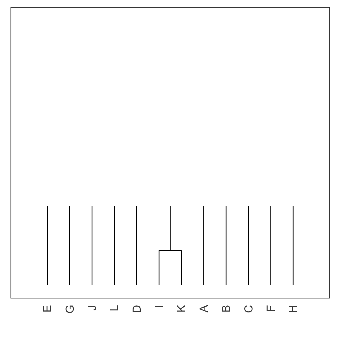
Single linkage demo: iteration 1
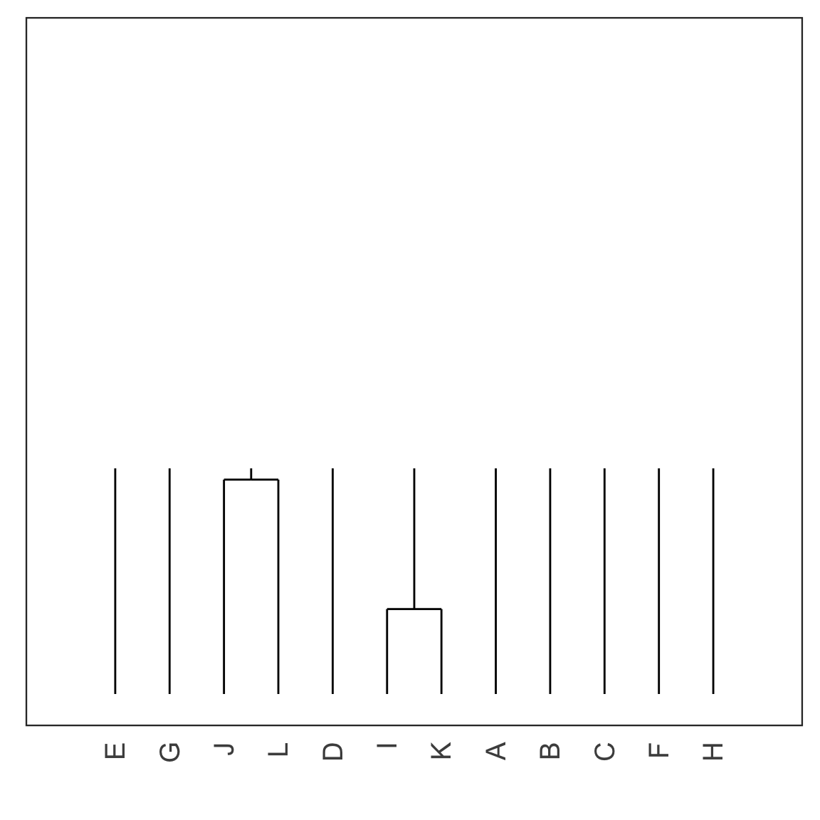
Single linkage demo: iteration 2
Single linkage demo: iteration 3
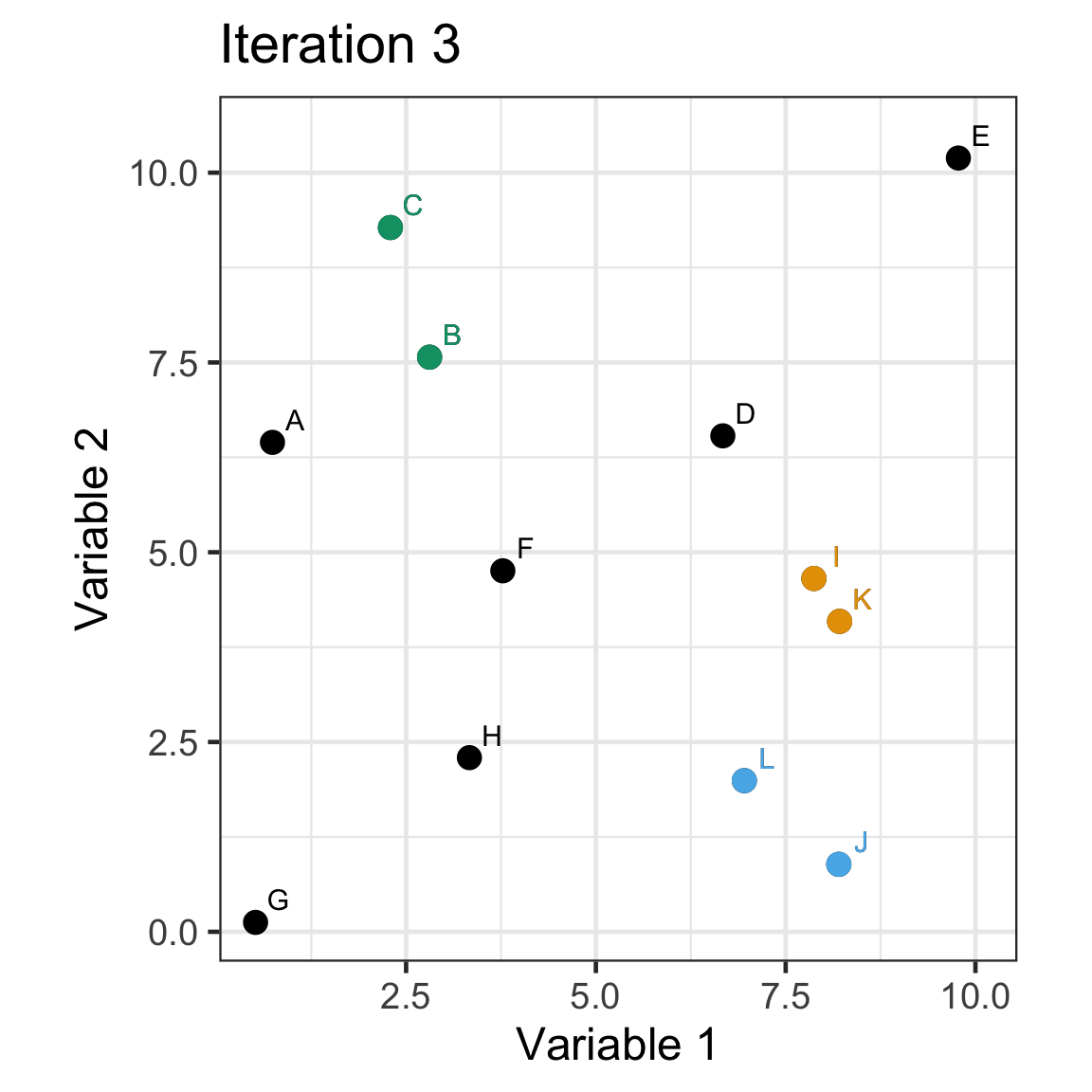
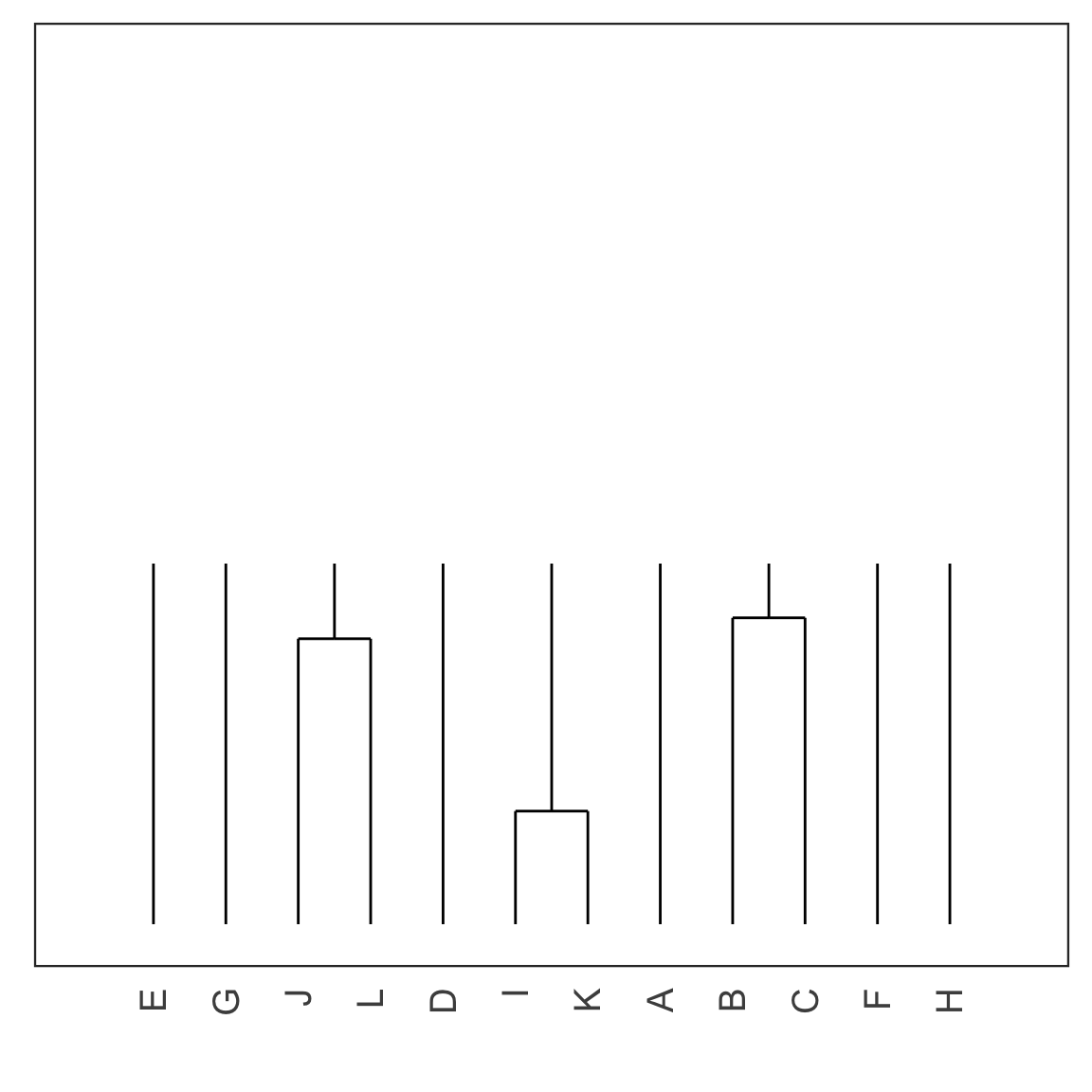
Single linkage demo: iteration 4

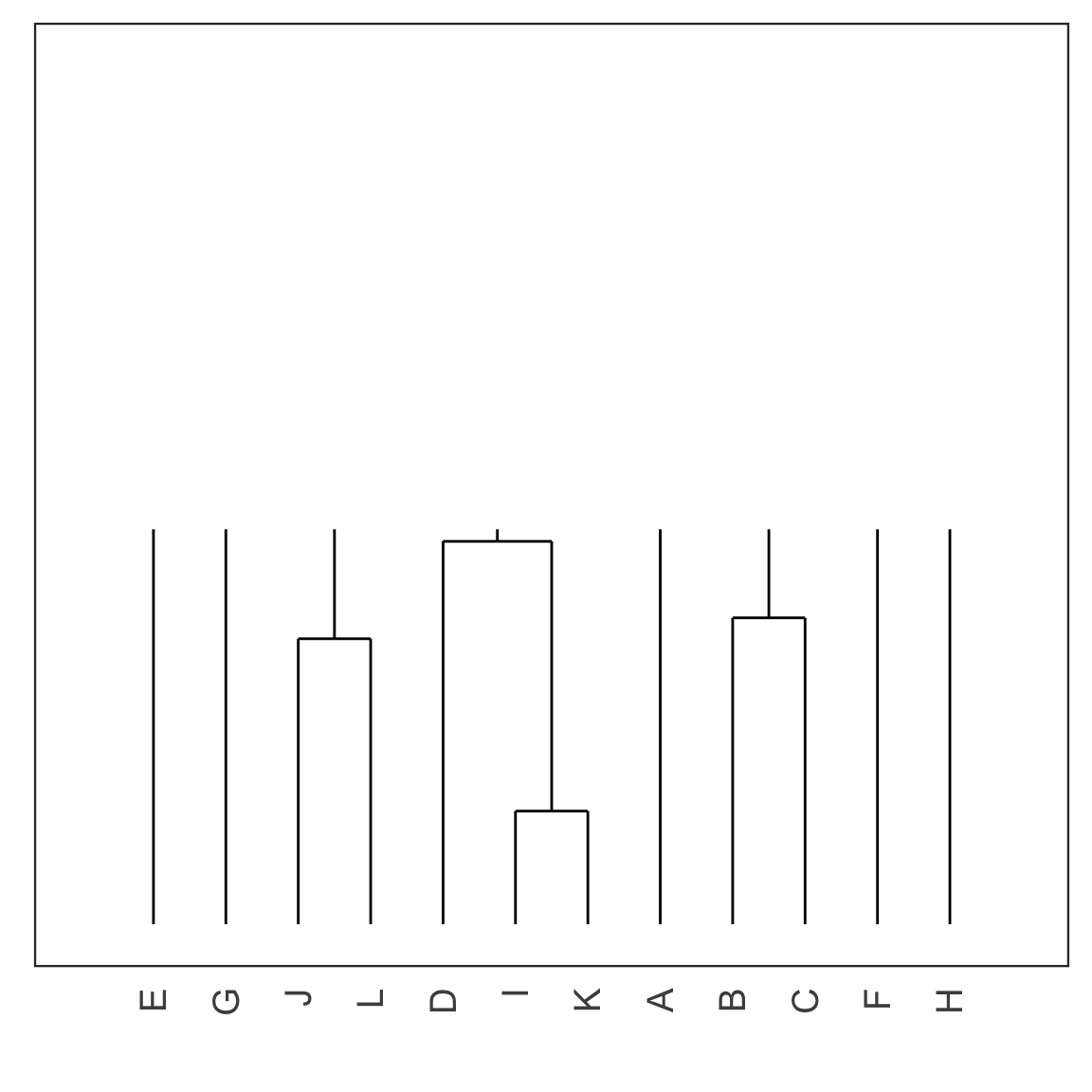
Single linkage demo: iteration 5
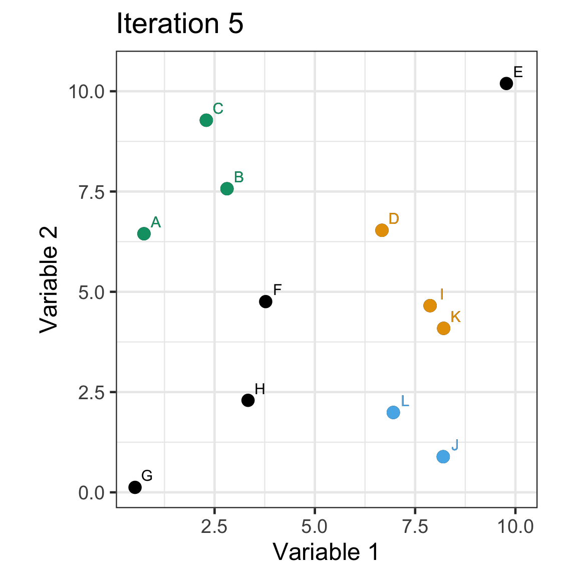
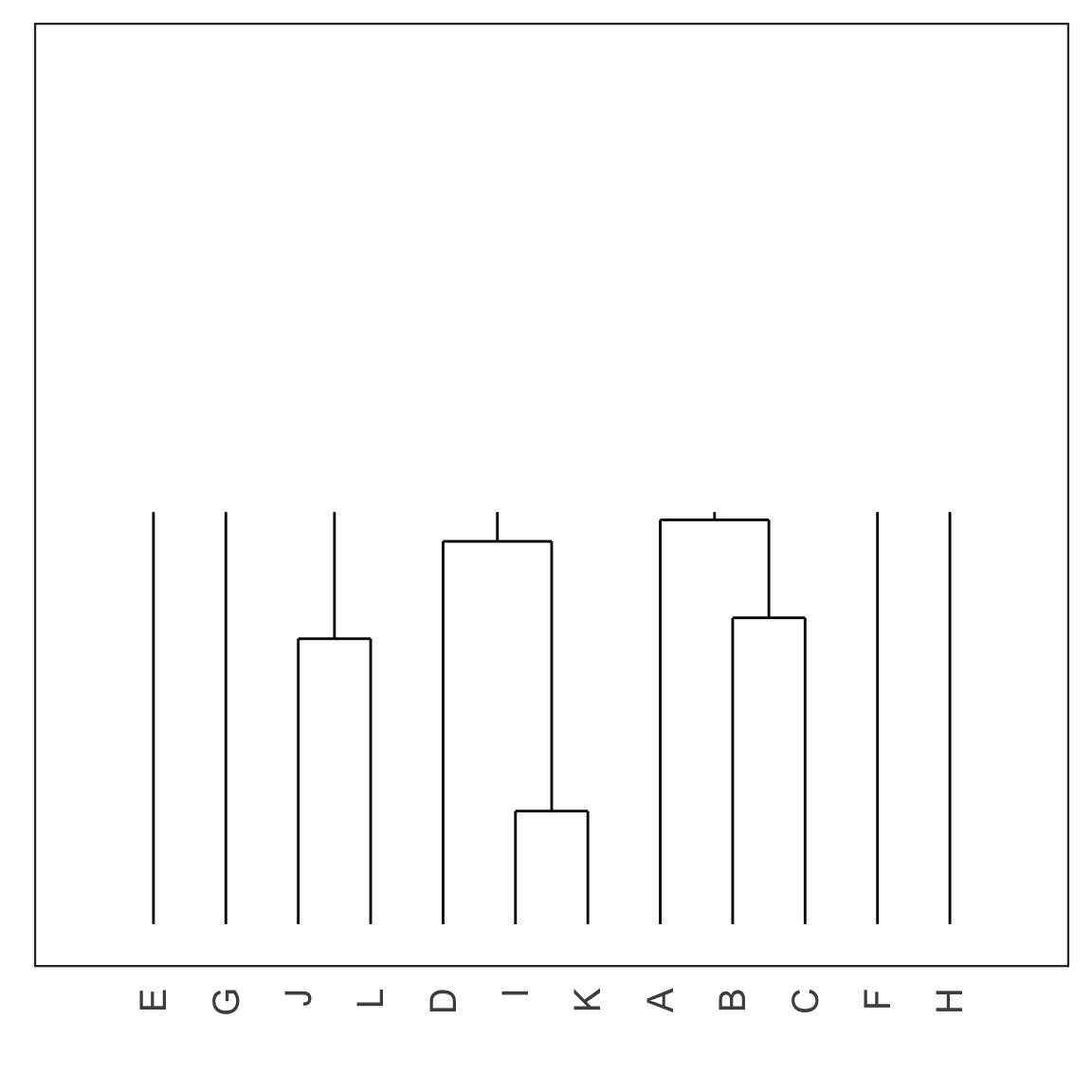
Single linkage demo: iteration 6
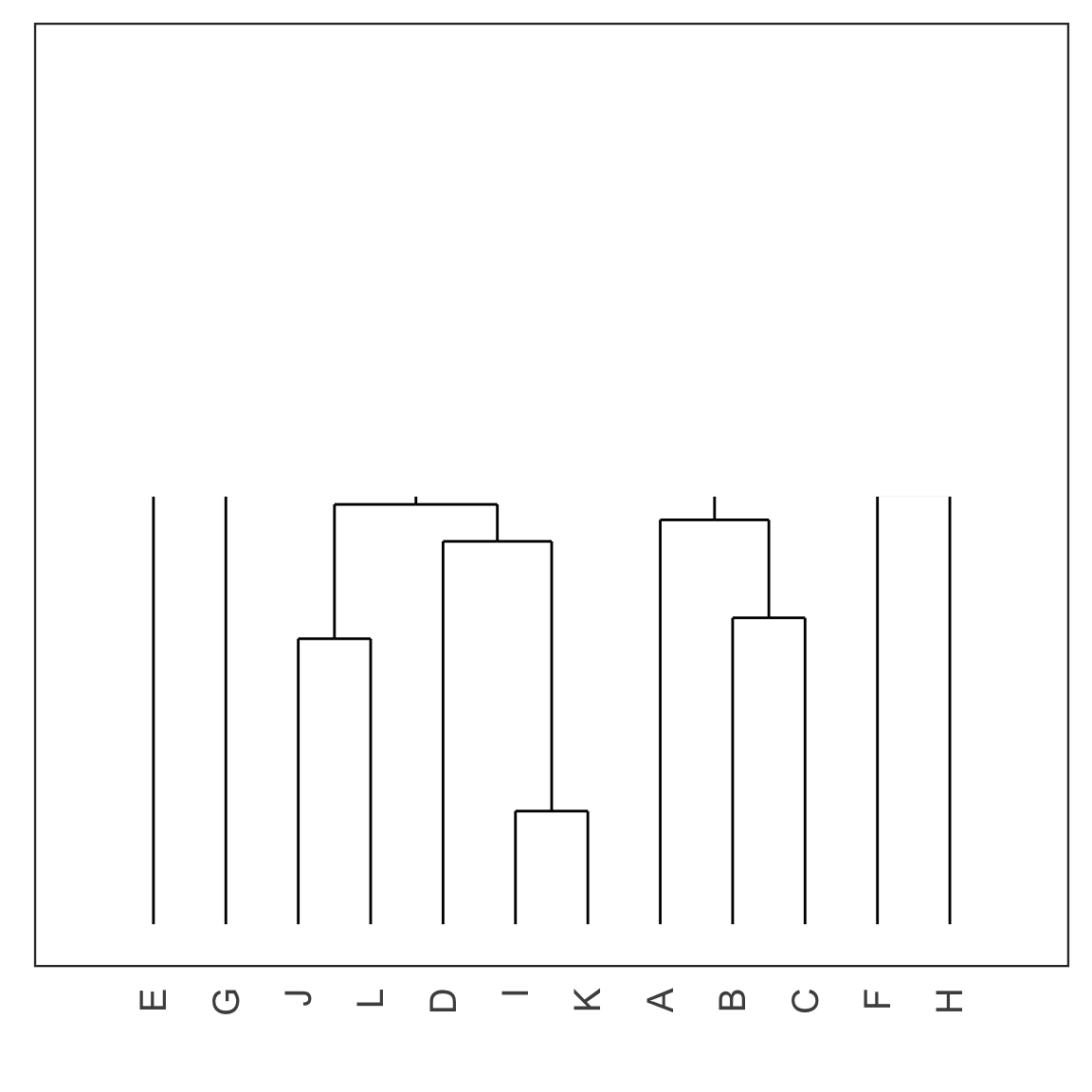
Single linkage demo: iteration 7
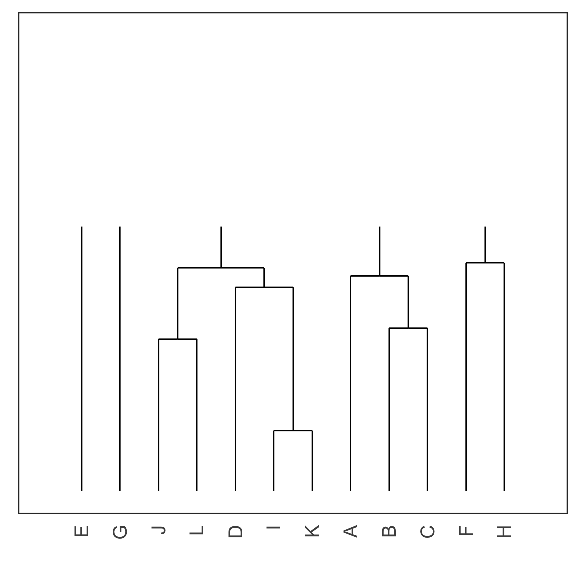
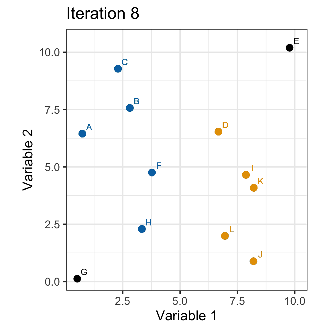
Single linkage demo: iteration 8
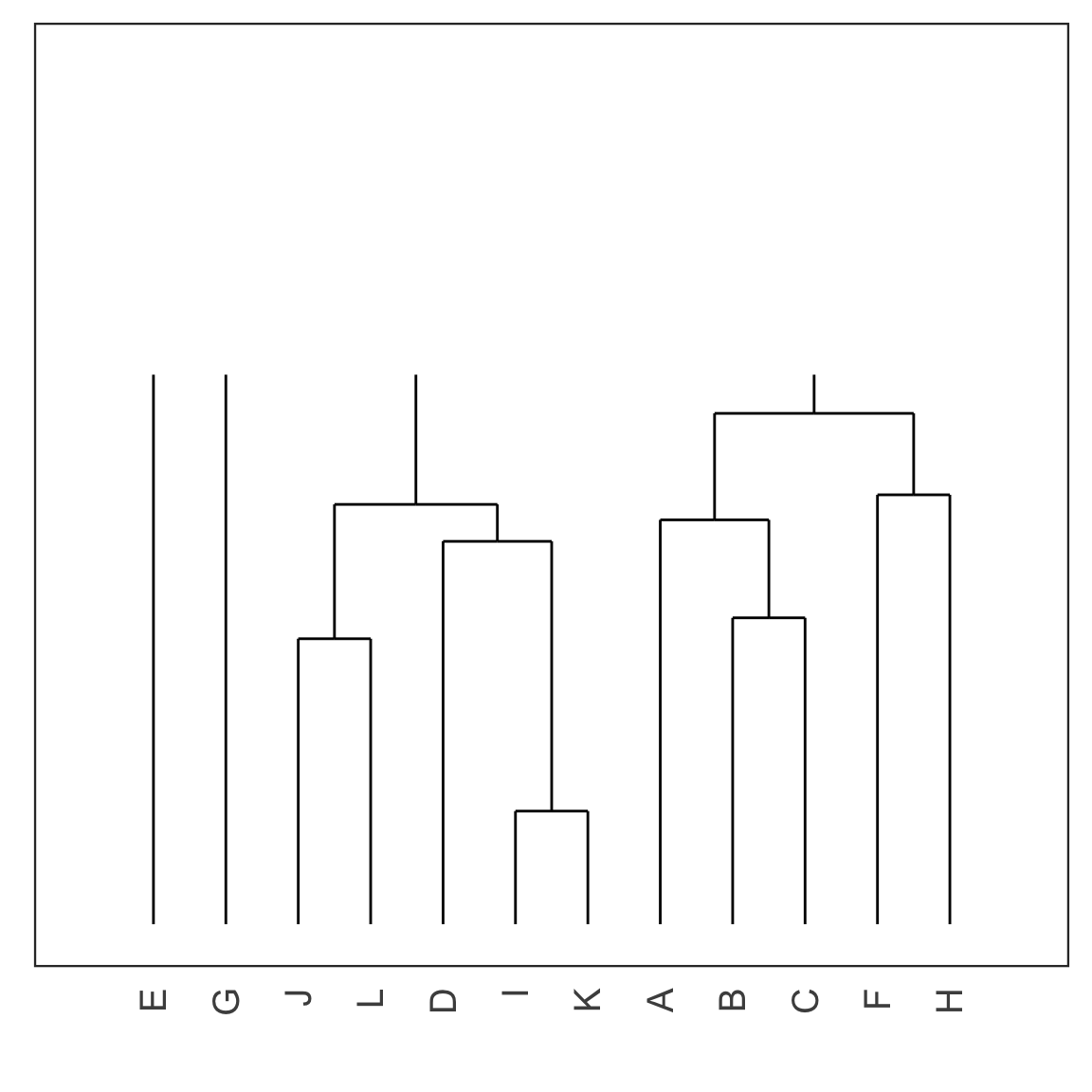
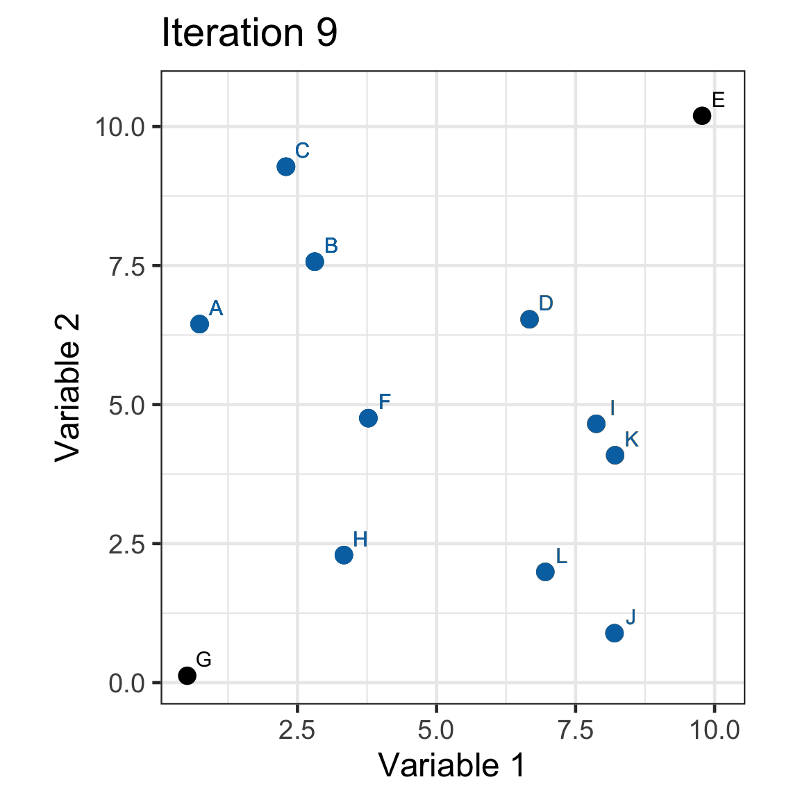
Single linkage demo: iteration 9
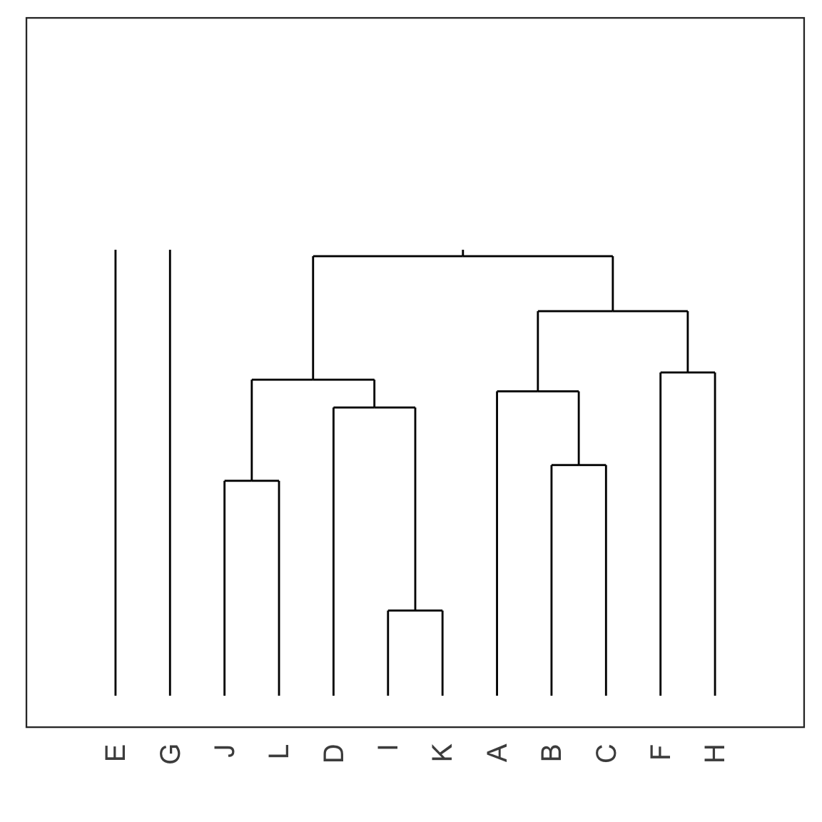
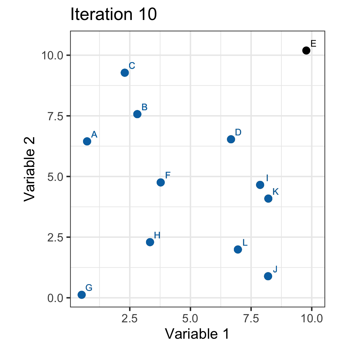
Single linkage demo: iteration 10
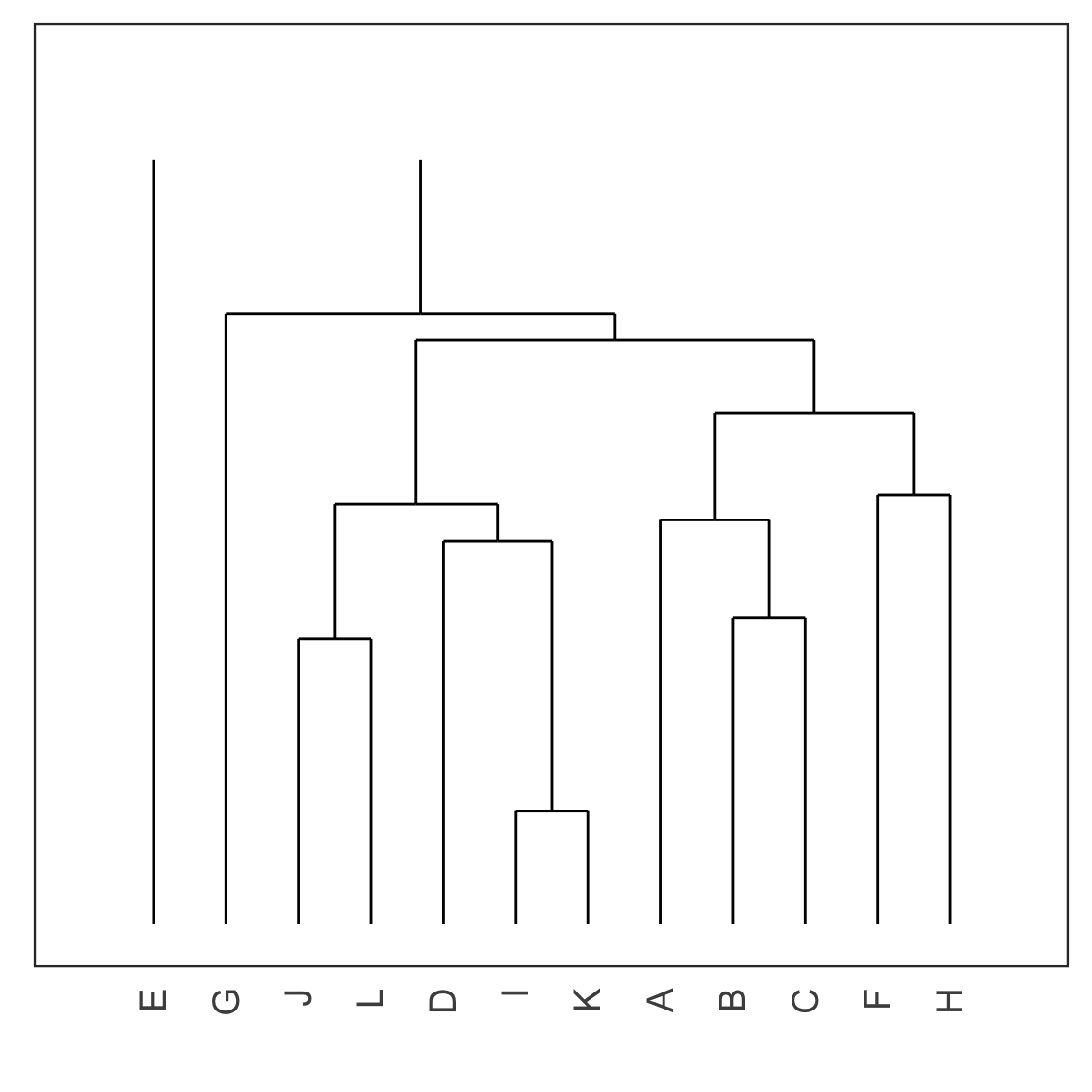
Single linkage demo: iteration 11
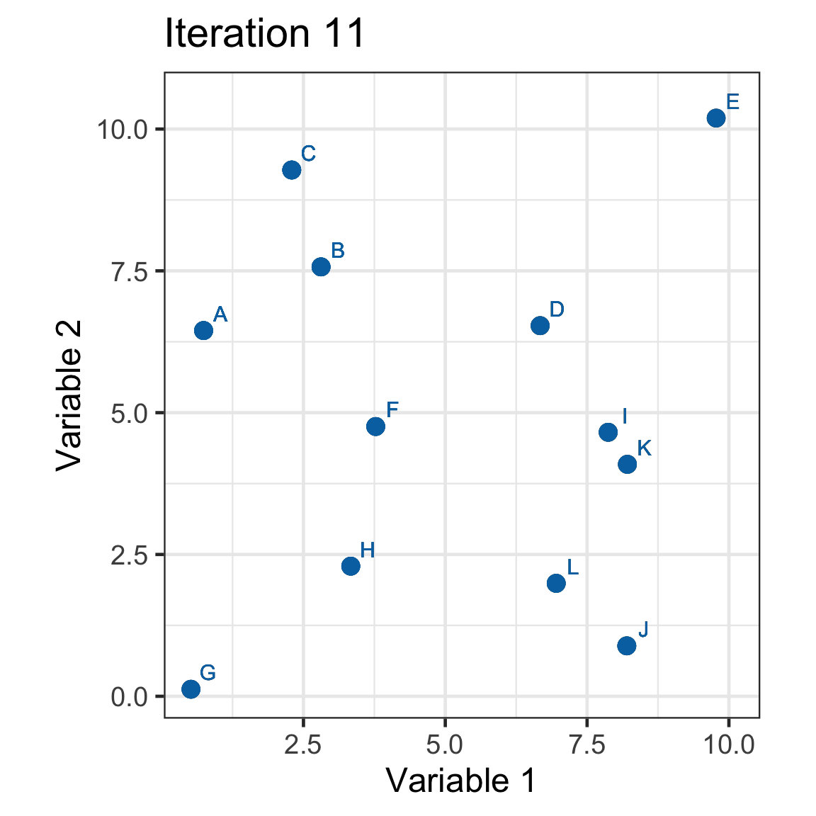
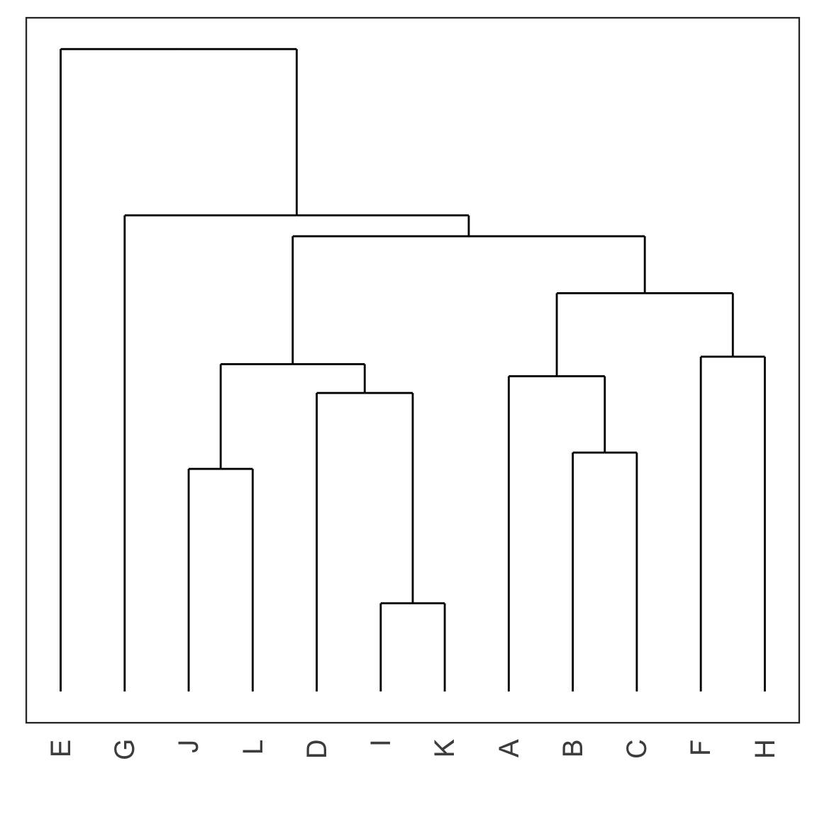
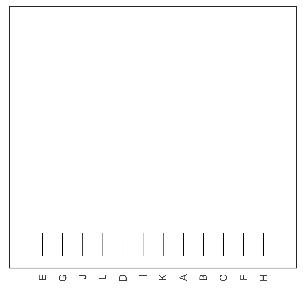
Dendrogram
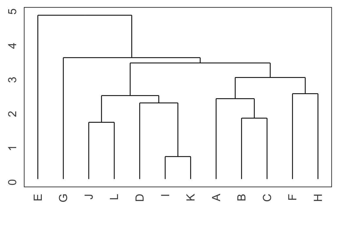
- Each leaf of the dendrogram represents one observation.
- Leaves fuse into branches and branches fuse, either with leaves or other branches.
- Fusions lower in the tree mean the groups of observations are more similar to each other.
Cutting the tree
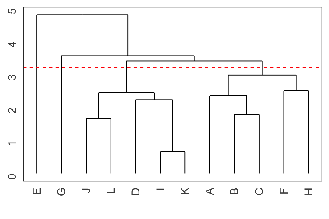
- Cut the tree at a particular height results in a particular set of clusters.
- For example, cutting the tree at the dashed red line below results in 4 clusters: (E), (G), (J, L, D, I K) and (A, B, C, F, H).
Chaining
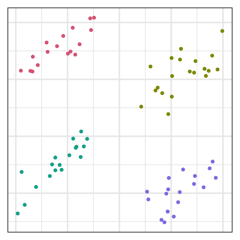
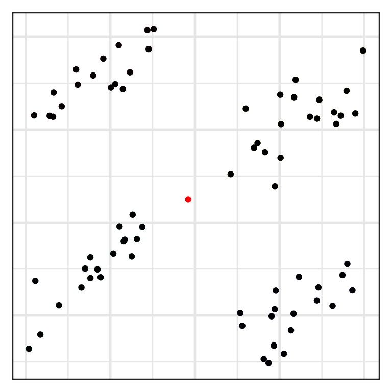
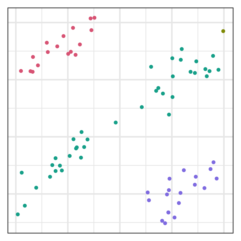
- Single linkage often suffers from chaining, i.e. a single observation results in merging two clusters.
- This results in clusters that are spread out and not compact.
Inlier and outlier
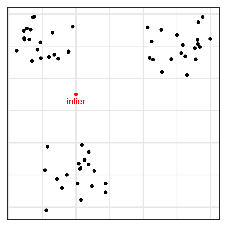
- An inlier is an erroneous observation that lies within the interior of a distribution.
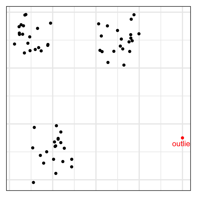
- An outlier is an observation that lies well outside the typical range of values.
Robustness
- Methods that are not often affected by single observations are referred to be robust.
- Single linkage is easily affected by inliers.
- Complete linkage less affected by inliers but affected by outliers.
- Other methods like average linkage, centroid linkage and Ward’s method are more robust.
Hierarchical clustering with R
Yale face database
Code
Sys.setenv(VROOM_CONNECTION_SIZE = 5000000)
yalefaces <- read_csv("https://emitanaka.org/iml/data/yalefaces.csv")

imagedata_to_plotdata <- function(data = yalefaces,
                                  w = 320,
                                  h = 243,
                                  which = sample(1:165, 15)) {
  data %>%
    mutate(id = 1:n()) %>%
    filter(id %in% which) %>%
    pivot_longer(starts_with("V")) %>%
    mutate(col = rep(rep(1:w, each = h), n_distinct(id)),
           row = rep(rep(1:h, times = w), n_distinct(id)))
}

gfaces <- imagedata_to_plotdata(yalefaces) %>%
    ggplot(aes(col, row)) +
    geom_tile(aes(fill = value)) +
    facet_wrap(~subject + type, nrow = 3) +
    scale_y_reverse() +
    theme_void(base_size = 18) +
    guides(fill = "none") +
    coord_equal()

gfaces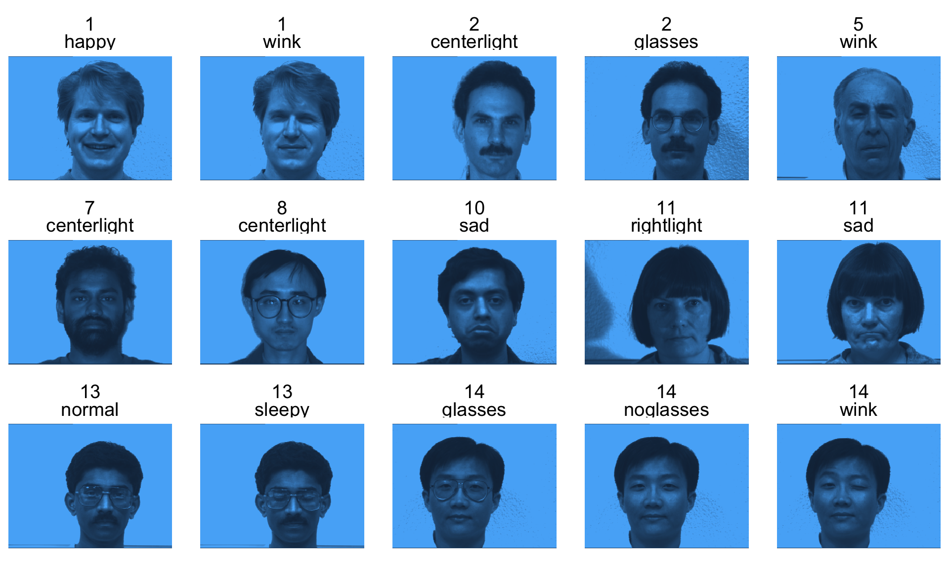
Principle components as features
- Applying hierarchical clustering with various methods:
hsingle <- hclust(dist(yalefaces_pca$x), method = "single")
hcomplete <- hclust(dist(yalefaces_pca$x), method = "complete")
haverage <- hclust(dist(yalefaces_pca$x), method = "average")
hcentroid <- hclust(dist(yalefaces_pca$x), method = "centroid")
hward <- hclust(dist(yalefaces_pca$x), method = "ward.D2")
# add labels
hsingle$labels <- paste("Subject", yalefaces$subject, yalefaces$type)
hcomplete$labels <- paste("Subject", yalefaces$subject, yalefaces$type)
haverage$labels <- paste("Subject", yalefaces$subject, yalefaces$type)
hcentroid$labels <- paste("Subject", yalefaces$subject, yalefaces$type)
hward$labels <- paste("Subject", yalefaces$subject, yalefaces$type)
Dendrogram with R
scroll
Cutting the tree with R
 Subject 1 centerlight      Subject 1 glasses        Subject 1 happy
                     1                      1                      1
   Subject 1 leftlight    Subject 1 noglasses       Subject 1 normal
                     2                      3                      1
  Subject 1 rightlight          Subject 1 sad       Subject 1 sleepy
                     4                      1                      1
   Subject 1 surprised         Subject 1 wink  Subject 2 centerlight
                     1                      1                      3
     Subject 2 glasses        Subject 2 happy    Subject 2 leftlight
                     3                      3                      2
   Subject 2 noglasses       Subject 2 normal   Subject 2 rightlight
                     3                      3                      5
         Subject 2 sad       Subject 2 sleepy    Subject 2 surprised
                     3                      3                      3
        Subject 2 wink  Subject 3 centerlight      Subject 3 glasses
                     3                      6                      6
       Subject 3 happy    Subject 3 leftlight    Subject 3 noglasses
                     7                      8                      7
      Subject 3 normal   Subject 3 rightlight          Subject 3 sad
                     7                      4                      7
      Subject 3 sleepy    Subject 3 surprised         Subject 3 wink
                     7                      7                      7
 Subject 4 centerlight      Subject 4 glasses        Subject 4 happy
                     5                      5                      5
   Subject 4 leftlight    Subject 4 noglasses       Subject 4 normal
                     2                      5                      5
  Subject 4 rightlight          Subject 4 sad       Subject 4 sleepy
                     4                      5                      5
   Subject 4 surprised         Subject 4 wink  Subject 5 centerlight
                     5                      5                      9
     Subject 5 glasses        Subject 5 happy    Subject 5 leftlight
                     9                      9                      2
   Subject 5 noglasses       Subject 5 normal   Subject 5 rightlight
                     9                      9                      4
         Subject 5 sad       Subject 5 sleepy    Subject 5 surprised
                     9                      9                      9
        Subject 5 wink  Subject 6 centerlight      Subject 6 glasses
                     9                     10                     11
       Subject 6 happy    Subject 6 leftlight    Subject 6 noglasses
                    11                      8                     11
      Subject 6 normal   Subject 6 rightlight          Subject 6 sad
                    11                     10                     11
      Subject 6 sleepy    Subject 6 surprised         Subject 6 wink
                    11                     11                     11
 Subject 7 centerlight      Subject 7 glasses        Subject 7 happy
                     6                      7                      6
   Subject 7 leftlight    Subject 7 noglasses       Subject 7 normal
                     8                      7                      7
  Subject 7 rightlight          Subject 7 sad       Subject 7 sleepy
                     4                      7                      7
   Subject 7 surprised         Subject 7 wink  Subject 8 centerlight
                     7                      7                      7
     Subject 8 glasses        Subject 8 happy    Subject 8 leftlight
                     7                      7                      8
   Subject 8 noglasses       Subject 8 normal   Subject 8 rightlight
                     7                      7                      4
         Subject 8 sad       Subject 8 sleepy    Subject 8 surprised
                     6                      7                      6
        Subject 8 wink  Subject 9 centerlight      Subject 9 glasses
                     6                      6                      6
       Subject 9 happy    Subject 9 leftlight    Subject 9 noglasses
                    12                      2                     12
      Subject 9 normal   Subject 9 rightlight          Subject 9 sad
                    12                      4                     12
      Subject 9 sleepy    Subject 9 surprised         Subject 9 wink
                    12                     12                     12
Subject 10 centerlight     Subject 10 glasses       Subject 10 happy
                     1                      6                     13
  Subject 10 leftlight   Subject 10 noglasses      Subject 10 normal
                     2                     13                     13
 Subject 10 rightlight         Subject 10 sad      Subject 10 sleepy
                     5                     13                     13
  Subject 10 surprised        Subject 10 wink Subject 11 centerlight
                    13                     13                     14
    Subject 11 glasses       Subject 11 happy   Subject 11 leftlight
                    14                     14                      8
  Subject 11 noglasses      Subject 11 normal  Subject 11 rightlight
                    14                     14                     14
        Subject 11 sad      Subject 11 sleepy   Subject 11 surprised
                    14                     14                     14
       Subject 11 wink Subject 12 centerlight     Subject 12 glasses
                    14                      3                      3
      Subject 12 happy   Subject 12 leftlight   Subject 12 noglasses
                     9                      2                      2
     Subject 12 normal  Subject 12 rightlight         Subject 12 sad
                     2                      3                      9
     Subject 12 sleepy   Subject 12 surprised        Subject 12 wink
                     9                      9                      9
Subject 13 centerlight     Subject 13 glasses       Subject 13 happy
                     6                     15                     15
  Subject 13 leftlight   Subject 13 noglasses      Subject 13 normal
                     8                     15                     15
 Subject 13 rightlight         Subject 13 sad      Subject 13 sleepy
                     4                     15                     15
  Subject 13 surprised        Subject 13 wink Subject 14 centerlight
                    15                     15                     10
    Subject 14 glasses       Subject 14 happy   Subject 14 leftlight
                    10                     10                      8
  Subject 14 noglasses      Subject 14 normal  Subject 14 rightlight
                    10                     10                     10
        Subject 14 sad      Subject 14 sleepy   Subject 14 surprised
                    10                     10                     10
       Subject 14 wink Subject 15 centerlight     Subject 15 glasses
                    10                      7                     13
      Subject 15 happy   Subject 15 leftlight   Subject 15 noglasses
                     6                      8                     13
     Subject 15 normal  Subject 15 rightlight         Subject 15 sad
                     7                      4                      6
     Subject 15 sleepy   Subject 15 surprised        Subject 15 wink
13 13 6 cward
1 2 3 4 5 6 7 8 9 10 11 12 13 14 15
9 9 13 9 11 14 22 8 14 12 8 7 11 10 8 Clustering results
scroll
Remember for the following we never used subject id variable in the clustering.
Cluster 1 is mostly subject 1!

- Cluster 2 seems to be capturing mostly the left light.

- Cluster 3 is mostly subject 2.
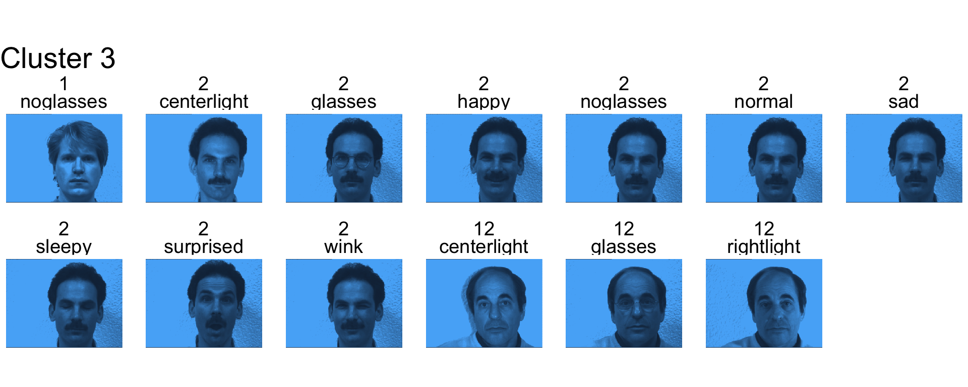
- Cluster 4 is mostly right light.

- Cluster 5 is mostly subject 4
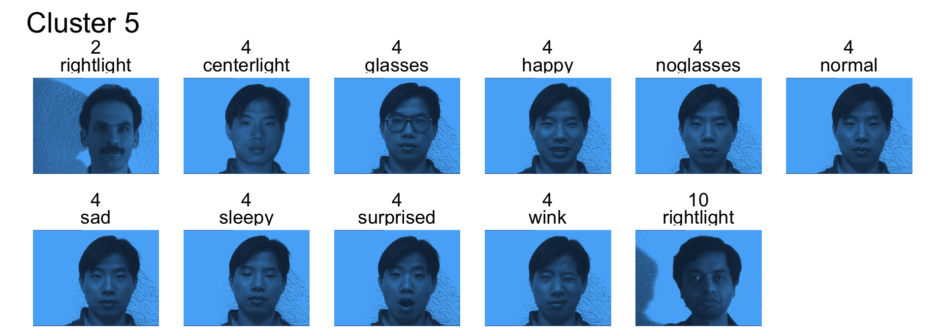
- Cluster 6 is a mix
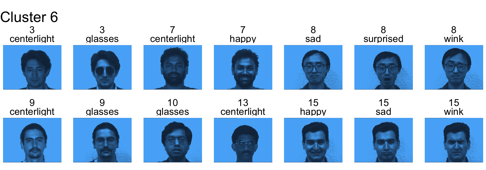
- Cluster 7 contains mostly subject 3, 7 and 8
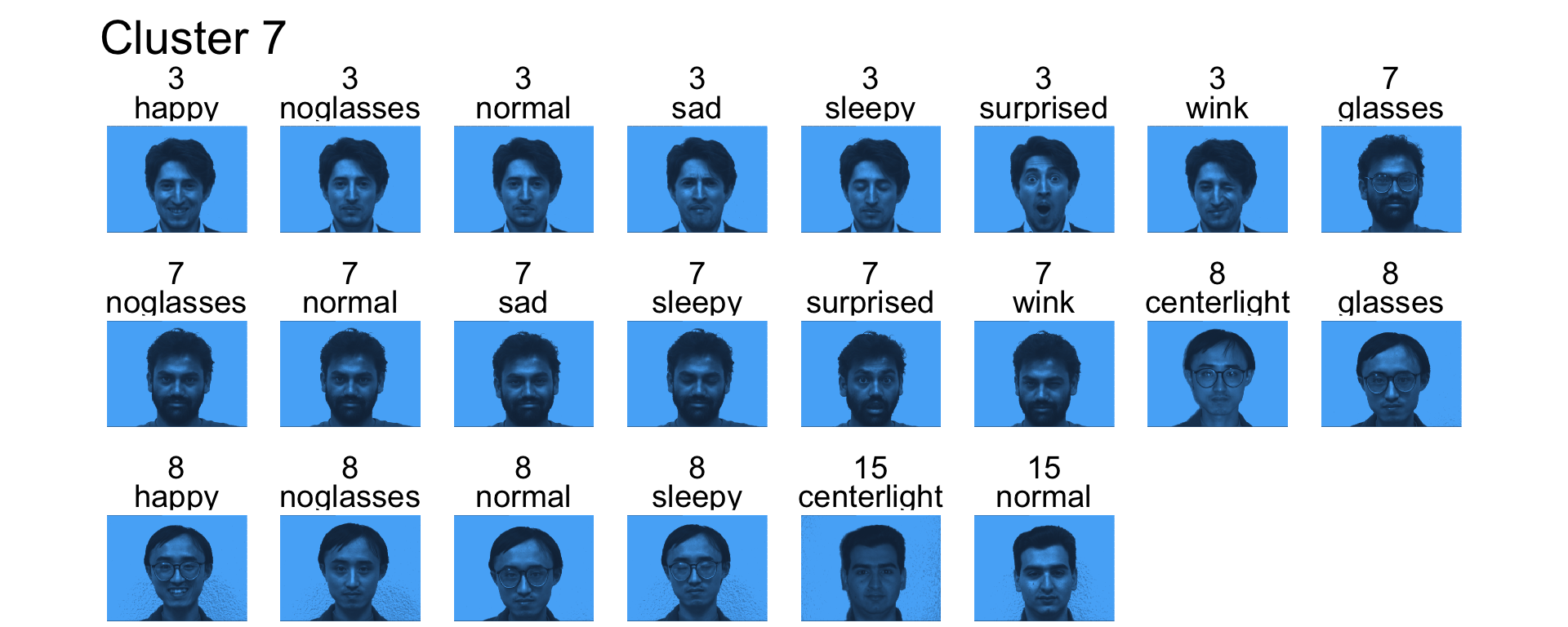
- Cluster 8 is the left light

- Cluster 9 is subjects 5 and 12
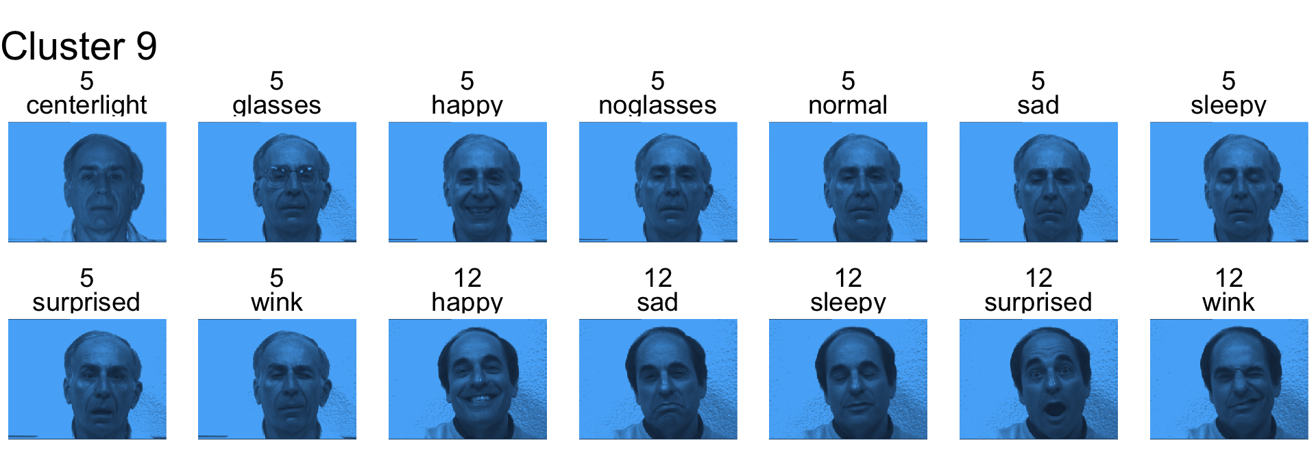
- Cluster 10 is mostly subject 14
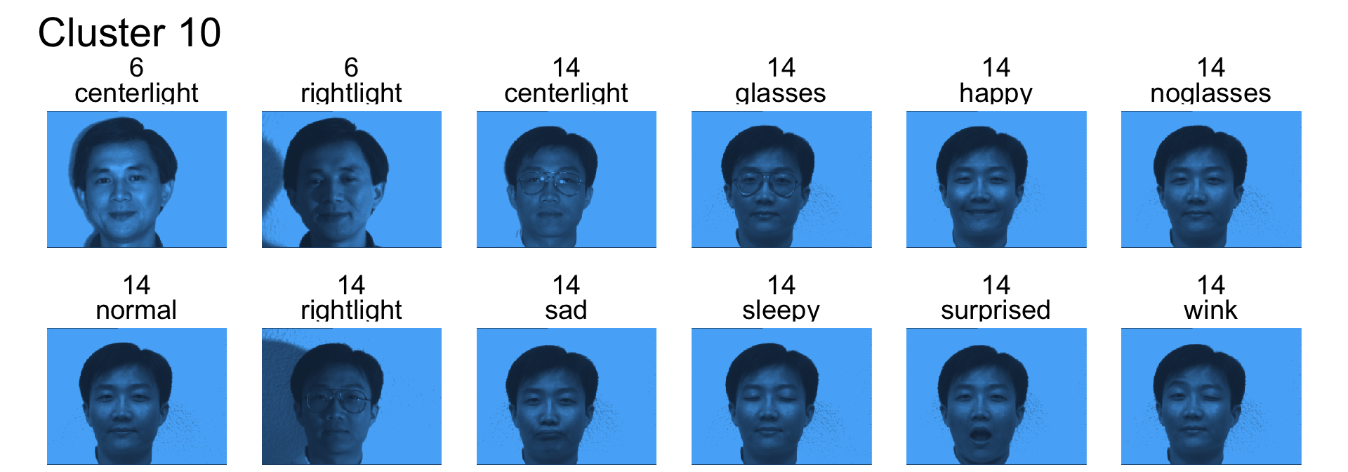
- Cluster 11 is subject 6

- Cluster 12 is subject 9

- Cluster 13 is subjects 10 and 15
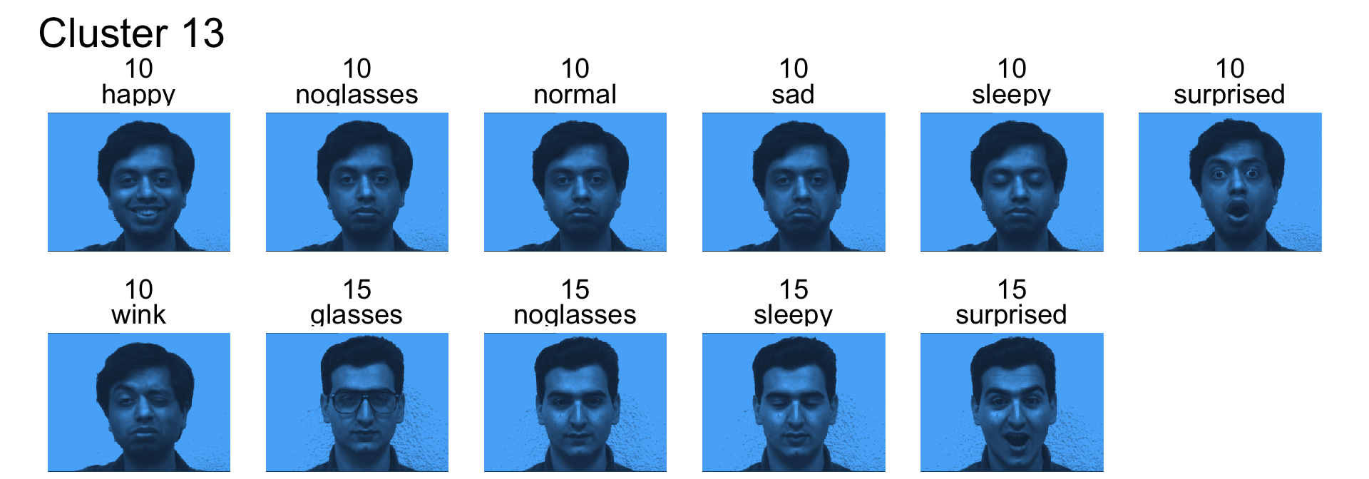
- Cluster 14 is subject 11
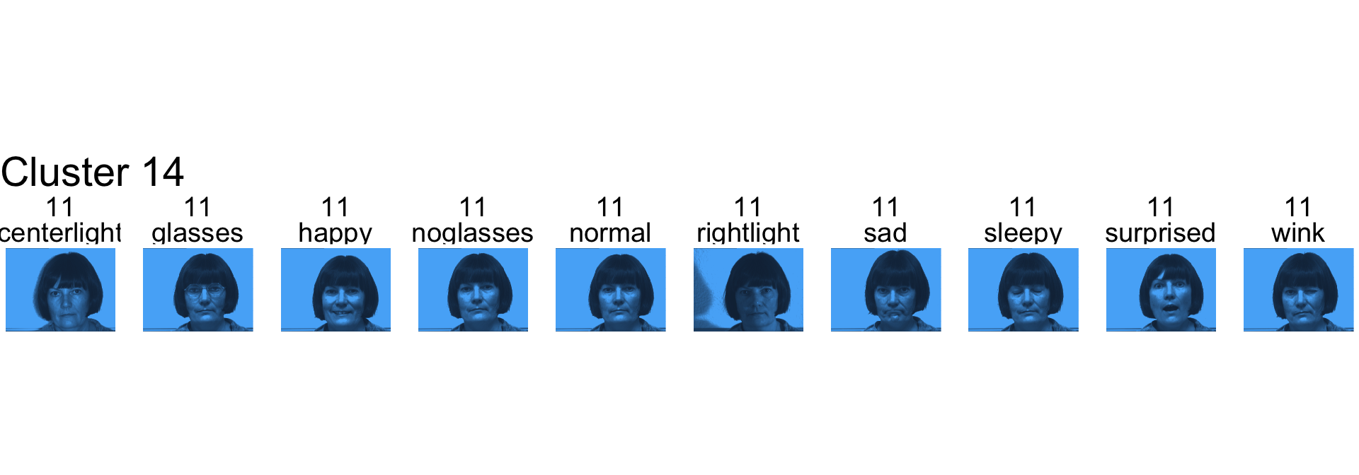
- Cluster 15 is subject 13

k-means clustering
k-means clustering algorithm
- The number of clusters, k, must be decided apriori to using this method.
- In k-means clustering, each observation must be closest to the centroid (or mean) of its own cluster.
- This method is iterative and follows along the lines of:
- Initially start with k partitions of data or k seed points.
- Assign observations to the cluster with the closest mean.
- Recompute centroids of each cluster.
- Repeat steps 2-3 until convergence.
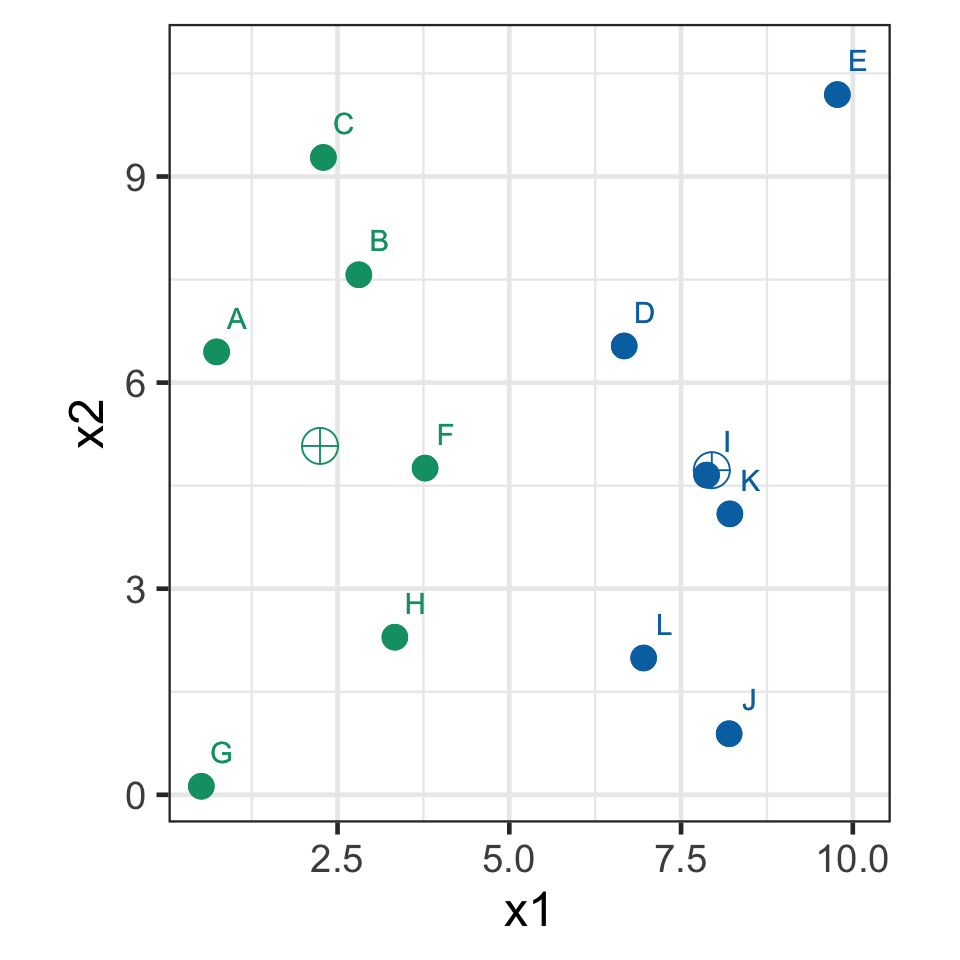
k-means demo: iteration 0
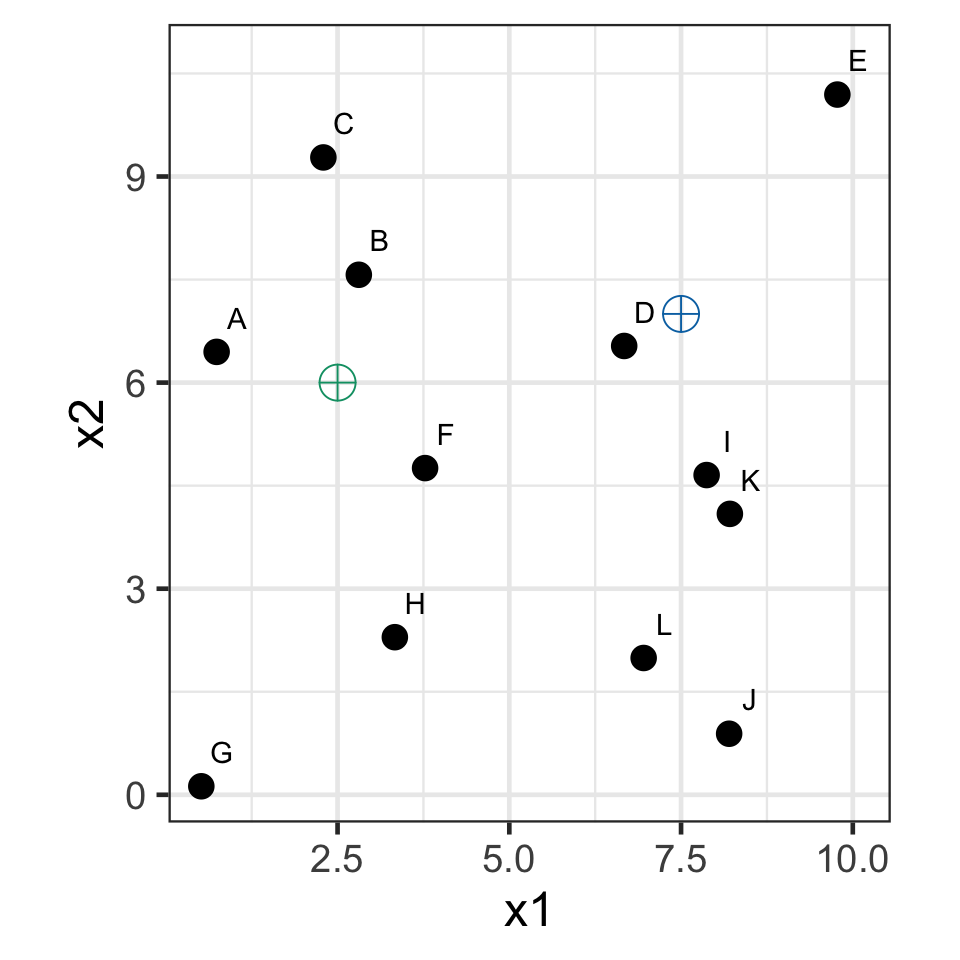
- Select k = 2 with initial seed points (2.5, 6) and (7.5, 7).
k-means demo: iteration 1
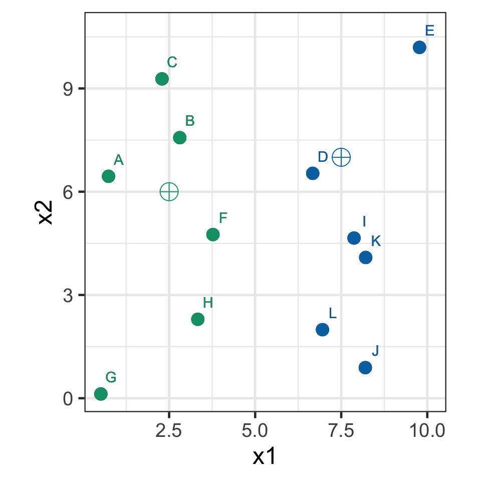
- Assign observations to the closest seed point.
k-means demo: iteration 2
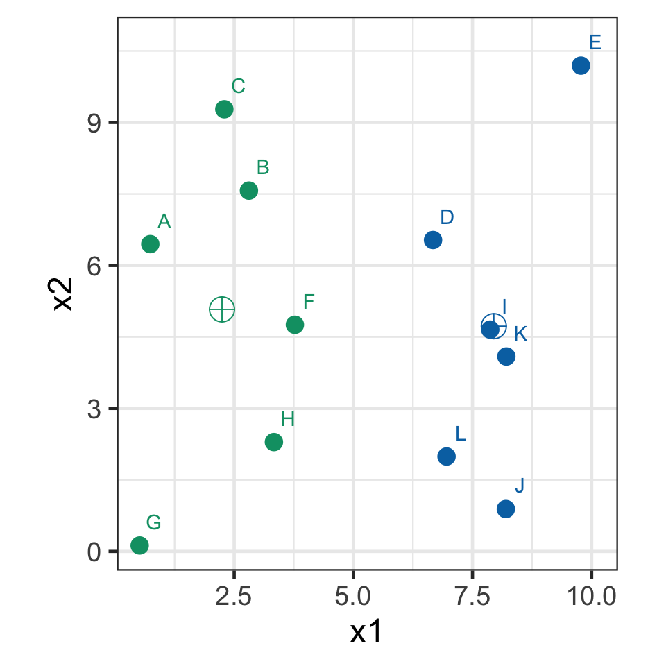
- Recompute the centroids.
k-means demo: iteration 3
- Assign observations to the closest centroid.
k-means clustering in R
kout <- kmeans(yalefaces_pca$x, centers = 15) # `scale` the data if different measurement units
str(kout)
List of 9
$ cluster : int [1:165] 12 12 12 8 4 12 11 12 12 12 ...
$ centers : num [1:15, 1:165] -6146 16755 -14911 -9669 22233 ...
..- attr(*, "dimnames")=List of 2
.. ..$ : chr [1:15] "1" "2" "3" "4" ...
.. ..$ : chr [1:165] "PC1" "PC2" "PC3" "PC4" ...
$ totss : num 5.63e+10
$ withinss : num [1:15] 8.93e+08 8.32e+08 5.04e+08 1.35e+09 5.06e+08 ...
$ tot.withinss: num 1.56e+10
$ betweenss : num 4.07e+10
$ size : int [1:15] 14 6 5 14 8 10 11 12 14 11 ...
$ iter : int 3
$ ifault : int 0
- attr(*, "class")= chr "kmeans"clustercontains the cluster number of the observation
Randomness in k-means clustering
- The k-means algorithm can yield quite different results depending on the initial seed.
k-means clustering caveats
- Unlike hierarchical clustering, the result for different number of clusters can contradict each other!
kout3 <- kmeans(yalefaces_pca$x, centers = 3)
kout5 <- kmeans(yalefaces_pca$x, centers = 5)
table(kout3$cluster, kout5$cluster)
     1  2  3  4  5
  1  0 47 14  0  5
  2 15  0  0  0 55
  3  0  0  0 29  0
hout3 <- cutree(hclust(dist(yalefaces_pca$x)), 3)
hout5 <- cutree(hclust(dist(yalefaces_pca$x)), 5)
table(hout3, hout5) hout5
hout3 1 2 3 4 5
1 76 0 0 43 0
2 0 17 0 0 0
3 0 0 9 0 20- k-means:
- 1\rightarrow 2, 3, 5
- 2\rightarrow 1, 5
- 3\rightarrow 4
- hierarchical:
- 1\rightarrow 1, 4
- 2\rightarrow 2
- 3\rightarrow 3, 5
Label switching
- Cluster labels can be switched around.
- Cluster 1 can be equivalent to Cluster 2 in another iteration – the number doesn’t matter.
koutA <- kmeans(yalefaces_pca$x, centers = 5)
koutB <- kmeans(yalefaces_pca$x, centers = 5)
table(koutA$cluster, koutB$cluster)
     1  2  3  4  5
  1 16 53  0  0  0
  2  6  0  0 44  0
  3  0  0  0  0 18
  4  0  0  0  0 11
5 0 0 17 0 0- Here Cluster 5 in A is Cluster 3 in B.
Takeaways
- Clustering is an unsupervised learning.
- There are many methods for clustering.
- Clustering helps to explore data.
- The choice of the number of clusters largely depends on the context of the problem – too many clusters may not be helpful but neither is too few.

ETC3250/5250 Week 9
