ETC3250/5250

Introduction to Machine Learning

Decision trees

Lecturer: Emi Tanaka

Department of Econometrics and Business Statistics

Classification trees

Classification tree

In a classification tree we use a recursive two-way partition (or branches) of predictors.

Classification trees with R

There are a number of R packages 📦 that can fit classification trees, e.g. tree and rpart.

Again, be sure to read the documentation and try fitting a model to toy data to check you know how it works.

Code for data

library(tidyverse)
cancer <- read_csv("https://emitanaka.org/iml/data/cancer.csv") %>% 
  mutate(diagnosis_binary = ifelse(diagnosis=="M", 1, 0),
         diagnosis = factor(diagnosis, levels = c("M", "B"))) %>% 
  janitor::clean_names()

library(rpart)
library(rsample)
set.seed(2023)
cancer_split <- initial_split(cancer)
cancer_train <- training(cancer_split)
cancer_rpart <- rpart(diagnosis ~ radius_mean + concave_points_mean, 
                      data = cancer_train,
                      method = "class")

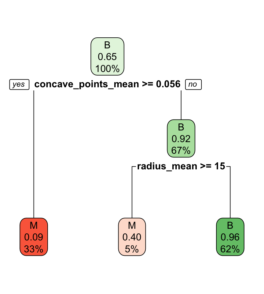
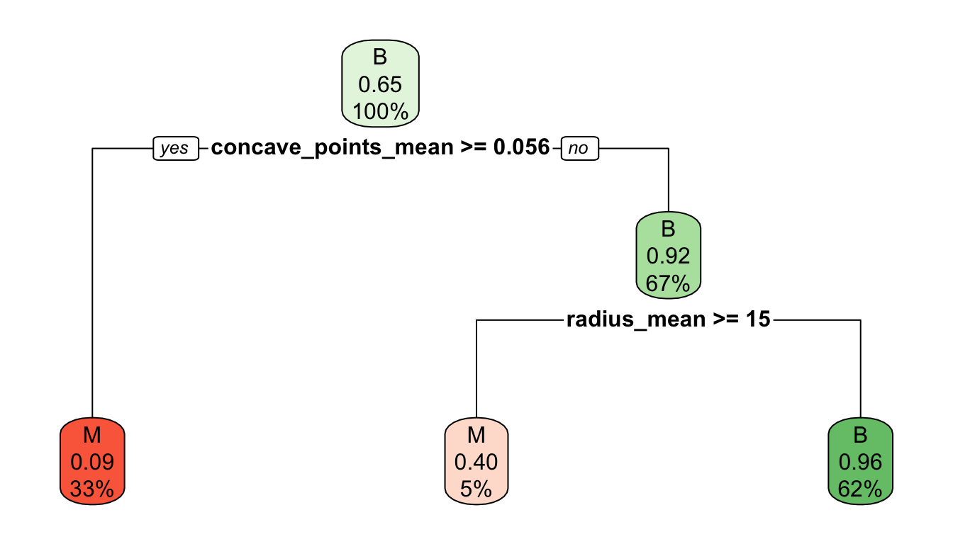
Interpreting classification tree plot

Code

library(rpart.plot)
rpart.plot(cancer_rpart, box.palette = "RdGn")

The rectangles are nodes that contain:
- class identifier,
- proportion of the reference class, and
- percentage of observations in node.
The bottom rectangles are terminal nodes (or leaves).
The bold text shows the splitting rules (branches).
Colors indicate class, with a darker color indicating lower impurity.

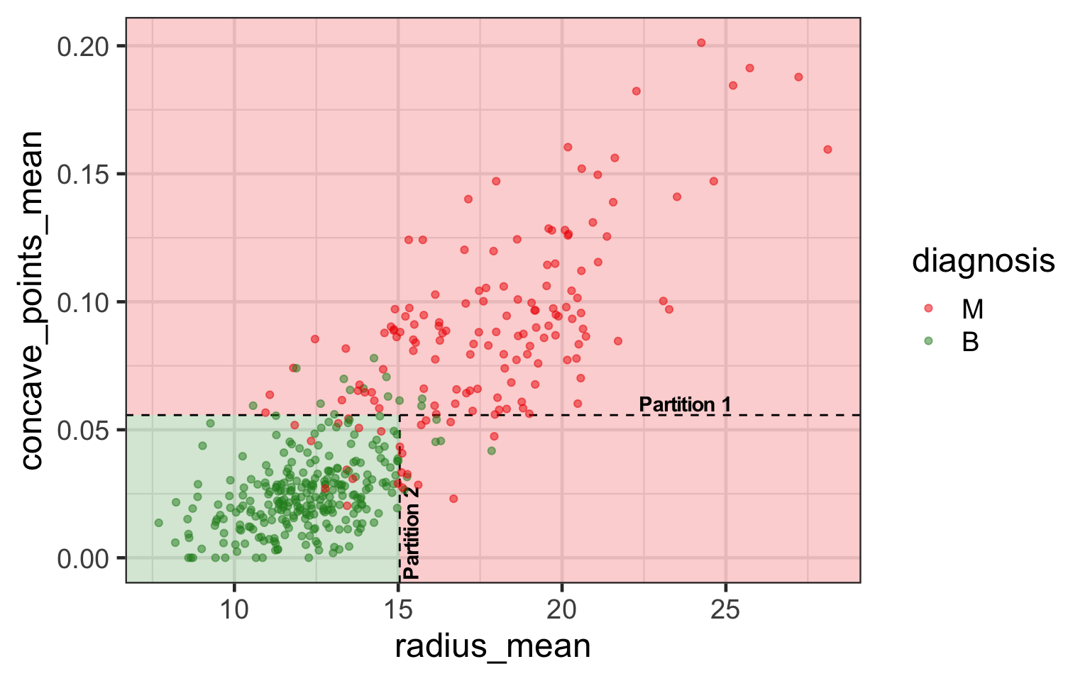
Classifying new observations

Code

library(rpart.plot)
rpart.plot(cancer_rpart, box.palette = "RdGn")

`id`	`concave_points_mean`	`radius_mean`
1	0.8	4.1
2	0.04	8.3
3	0.005	18.1

What class would above observations belong to according to this tree?

Partition notation

Suppose s is the value to split in variable j.
Then we have two sets (or nodes):
- \color{#C8008F}{\mathcal{A}_L} = \{\{y_i, \boldsymbol{x}_i\}:x_{ij}<s\} and
- \color{#027EB6}{\mathcal{A}_R} = \{\{y_i, \boldsymbol{x}_i\}:x_{ij}\geq s\}.
Different choices of j and s encode different partitions.
Suppose p_{k\mathcal{A}} is the proportion of observations in class k in a set \mathcal{A}.

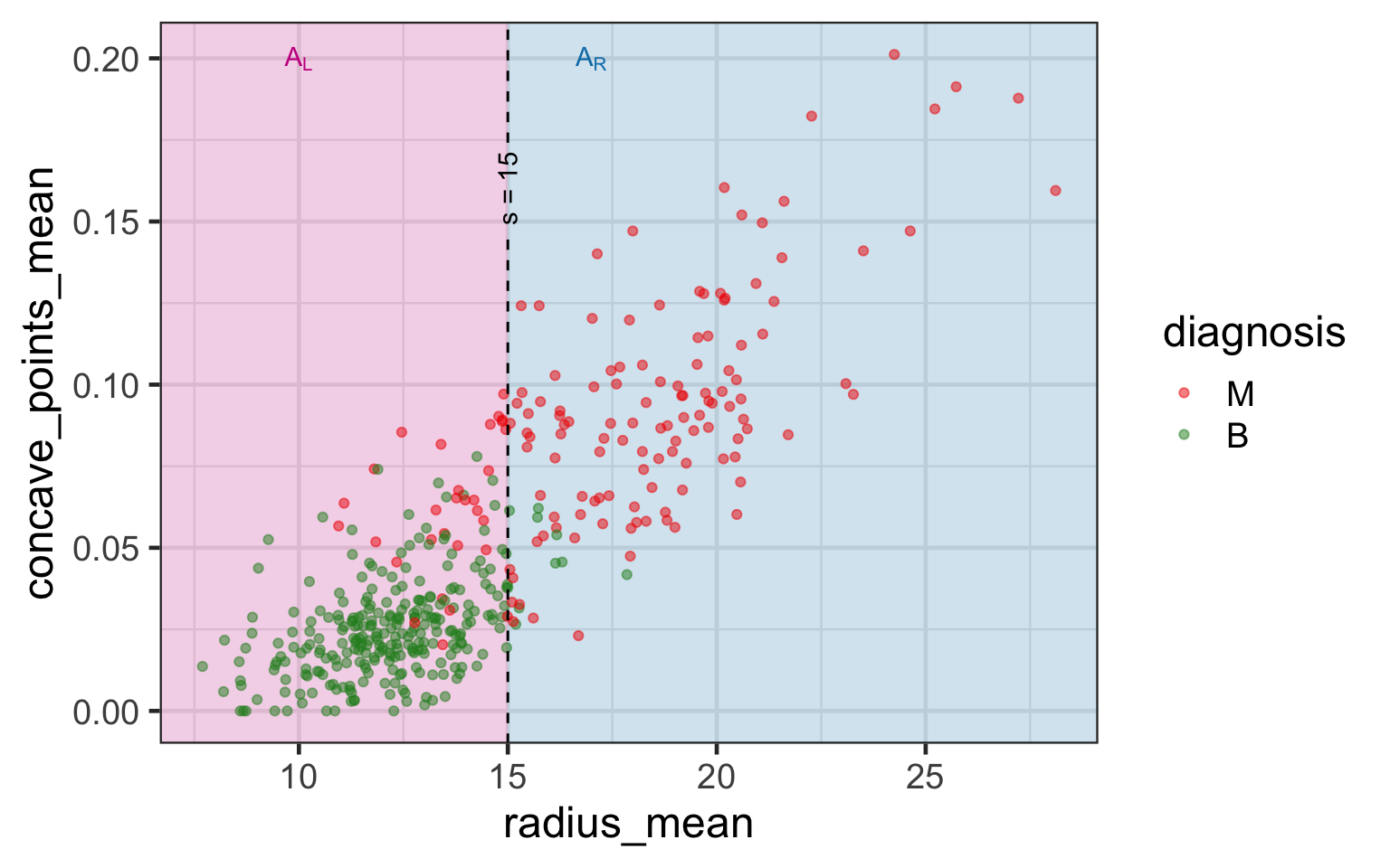
	\mathcal{A}_L	\mathcal{A}_R
p_{M}	10.2% (30)	92.4% (121)
p_{B}	89.8% (265)	7.6% (10)

Impurity metrics

We need an algorithm to find the optimal \{j^*, s^*\}.
Some popular impurity metrics are the:
- Gini index: f_{Gini}(\mathcal{A})= \sum_{k = 1}^K p_{k\mathcal{A}}(1 - p_{k\mathcal{A}}) = 1 - \sum_{k = 1}^K p_{k\mathcal{A}}^2
- entropy index: f_{entropy}(\mathcal{A}) = -\sum_{k = 1}^K p_{k\mathcal{A}}\log_2(p_{k\mathcal{A}}).
Smaller values of the impurity index means higher purity.
An overall impurity can be calculated from the weighted average: \frac{|\mathcal{A}_L|}{|\mathcal{A}_L| + |\mathcal{A}_R|}f(\mathcal{A}_L) + \frac{|\mathcal{A}_R|}{|\mathcal{A}_L| + |\mathcal{A}_R|}f(\mathcal{A}_R).

Example calculation of Gini impurity index

	\mathcal{A}_L	\mathcal{A}_R
p_{M}	10.2% (30)	92.4% (121)
p_{B}	89.8% (265)	7.6% (10)

f_{Gini}(\mathcal{A}_L) = 1 - \frac{(30^2 + 265^2)}{(30 + 265)^2} \approx 0.183
f_{Gini}(\mathcal{A}_R) = 1 - \frac{(121^2 + 10^2)}{(121 + 10)^2} \approx 0.141
\text{Overall impurity} = \frac{30 + 265}{30 + 265 + 121 + 10} 0.183 + \frac{121 + 10}{30 + 265 + 121 + 10} 0.141 \approx 0.17

Search for the optimal partition

The goal is to find j and s such that it minimises the overall impurity: \{j^*, s^*\} = \underset{j\in \{1, \dots, p\}, s \in \mathbb{R}}{\text{argmin}}~\text{Overall impurity}(\mathcal{A}_L, \mathcal{A}_R).

Selected partition

Selected predictor: j^* = \texttt{concave\_points\_mean}
Selected threshold: s^* = 0.056

Search for the next optimal partition

We find the next j and s such that it minimises the overall impurity for the partitioned subset.

We repeat again for the next subset and so on …
until we reach the stopping rule.

Stopping rules

The partitioning will be recursively applied until it meets the selected stopping rule.
Some stopping rules in rpart.control() include:
- minsplit: the minimum number of observations in any non-terminal node.
- minbucket: the minimum number of observations allowed in a terminal node.
- cp: complexity parameter – minimum difference between impurity values required to continue splitting.

Changing the stopping rules in `rpart`

cancer_rpart_stop <- rpart(diagnosis ~ radius_mean + concave_points_mean,
                           data = cancer_train, method = "class",
                           control = rpart.control(minbucket = 0.03 * nrow(cancer),
                                                   minsplit = 10,
                                                   cp = 0))

rpart.plot(cancer_rpart_stop, box.palette = "RdGn")

Algorithm in a nutshell

Start with all observations in a single set.
Sort values on first variable.
Compute overall impurity for all possible partitions into two sets.
Choose the best partition on this variable.
Repeat 2-4 for all other variables.
Choose the best partition among all variables. Your data is now split into two subsets.
Repeat 1-6 on each subset.
Stop when stopping rule is achieved.

Tuning parameters: search space

First we define the search space of the parameters.

search_df <- expand_grid(minbucket = seq(10, 100, length.out = 4),
                         minsplit = seq(10, 100, length.out = 4),
                         cp = seq(0, 1, length.out = 50)) 
search_df

# A tibble: 800 × 3
   minbucket minsplit     cp
       <dbl>    <dbl>  <dbl>
 1        10       10 0     
 2        10       10 0.0204
 3        10       10 0.0408
 4        10       10 0.0612
 5        10       10 0.0816
 6        10       10 0.102 
 7        10       10 0.122 
 8        10       10 0.143 
 9        10       10 0.163 
10        10       10 0.184 
# ℹ 790 more rows

Tuning parameters: fit and predict

scroll

library(yardstick)
set.seed(2023)
cancer_folds <- cancer_train %>% 
  vfold_cv(v = 5) 

search_res <- cancer_folds %>% 
  mutate(search = map(splits, function(asplit) {
    search_df %>% 
      rowwise() %>% 
      # fit the model for each row 
      # different row contains unique combination of 
      # minbucket, minsplit, and cp
      mutate(fit = list(rpart(diagnosis ~ radius_mean + concave_points_mean,
                              data = training(asplit), method = "class",
                              control = rpart.control(minbucket = .data$minbucket,
                                                      minsplit = .data$minsplit,
                                                      cp = .data$cp)))) %>% 
      ungroup() %>% 
      # compute classification metric on validation fold
      mutate(metrics = map(fit, function(afit) {
        # get validation fold
        testing(asplit) %>% 
          # predict from fitted model for this validation fold
          mutate(pred = predict(afit, ., type = "class")) %>% 
          # get classification metrics
          metric_set(accuracy, bal_accuracy, kap)(., truth = diagnosis, estimate = pred)
      })) %>% 
      unnest(metrics) %>% 
      select(-c(fit, .estimator))
  })) %>% 
  unnest(search)

# summarise the data for easy view
search_res_summary <- search_res %>% 
  group_by(minbucket, minsplit, cp, .metric) %>% 
  summarise(mean = mean(.estimate),
            sd = sd(.estimate))

search_res_summary

# A tibble: 2,400 × 6
# Groups:   minbucket, minsplit, cp [800]
   minbucket minsplit     cp .metric       mean     sd
       <dbl>    <dbl>  <dbl> <chr>        <dbl>  <dbl>
 1        10       10 0      accuracy     0.906 0.0275
 2        10       10 0      bal_accuracy 0.896 0.0366
 3        10       10 0      kap          0.794 0.0583
 4        10       10 0.0204 accuracy     0.904 0.0409
 5        10       10 0.0204 bal_accuracy 0.900 0.0417
 6        10       10 0.0204 kap          0.792 0.0864
 7        10       10 0.0408 accuracy     0.897 0.0314
 8        10       10 0.0408 bal_accuracy 0.886 0.0260
 9        10       10 0.0408 kap          0.774 0.0633
10        10       10 0.0612 accuracy     0.899 0.0306
# ℹ 2,390 more rows

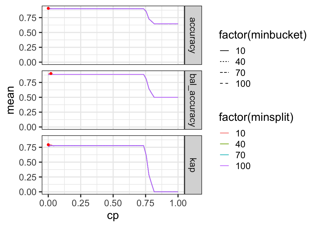
Tuning parameters: results

Code

search_res_summary_max <- search_res_summary %>% 
  group_by(.metric) %>% 
  filter(mean == max(mean))

search_res_summary %>% 
  ggplot(aes(cp, mean)) +
  geom_line(aes(color = factor(minsplit), linetype = factor(minbucket))) + 
  geom_point(data = search_res_summary_max,
             color = "red") +
  facet_grid(.metric ~ .)

minbucket	minsplit	cp	.metric	mean	sd
10	10	0.0000000	accuracy	0.9061286	0.0274646
10	10	0.0000000	kap	0.7935643	0.0583496
10	10	0.0204082	bal_accuracy	0.9004277	0.0417005

minbucket and minsplit doesn’t seem to make much difference (for the range searched at least).
cp = 0 seems sufficient in this case.

Tuning `cp` with cross validation error in `rpart`

rpart automatically stores the cross validation error in the resulting model object

fit <- rpart(diagnosis ~ radius_mean + concave_points_mean,
             data = cancer_train, method = "class",
             control = rpart.control(cp = 0, xval = 10)) # 10 folds (default)
fit$cptable

           CP nsplit rel error    xerror       xstd
1 0.768211921      0 1.0000000 1.0000000 0.06538424
2 0.026490066      1 0.2317881 0.2781457 0.04074821
3 0.006622517      2 0.2052980 0.2715232 0.04031258
4 0.000000000      3 0.1986755 0.2847682 0.04117673

rel error is the in-sample error (always decreases with more split)
xerror is the cross-validation error
xstd is the standard deviation of the cross-validation error

Bank marketing data

scroll

This data found here contains direct marketing campaigns of a Portuguese banking institution.
🎯 The goal is to predict if the client will subscribe to a term deposit (y = "yes" or "no").

library(tidyverse)
bank <- read_delim("https://emitanaka.org/iml/data/bank-full.csv", delim = ";")
skimr::skim(bank)

Data summary
Name	bank
Number of rows	45211
Number of columns	17
_______________________
Column type frequency:
character	10
numeric	7
________________________
Group variables	None

Variable type: character

skim_variable	complete_rate	min	max	n_unique
job	1	6	13	12
marital	1	6	8	3
education	1	7	9	4
default	1	2	3	2
housing	1	2	3	2
loan	1	2	3	2
contact	1	7	9	3
month	1	3	3	12
poutcome	1	5	7	4
y	1	2	3	2

Variable type: numeric

skim_variable	complete_rate	mean	sd	p0	p25	p50	p75	p100	hist
age	1	40.94	10.62	18	33	39	48	95	▅▇▃▁▁
balance	1	1362.27	3044.77	-8019	72	448	1428	102127	▇▁▁▁▁
day	1	15.81	8.32	1	8	16	21	31	▇▆▇▆▆
duration	1	258.16	257.53	0	103	180	319	4918	▇▁▁▁▁
campaign	1	2.76	3.10	1	1	2	3	63	▇▁▁▁▁
pdays	1	40.20	100.13	-1	-1	-1	-1	871	▇▁▁▁▁
previous	1	0.58	2.30	0	0	0	0	275	▇▁▁▁▁

Fitting and visualising the model

duration is omitted as a predictor in the model as it is computed based on the response.

fit_rpart <- rpart(y ~ . - duration, data = bank, method = "class")
rpart.plot(fit_rpart)

How are partitions determined for categorical variables?

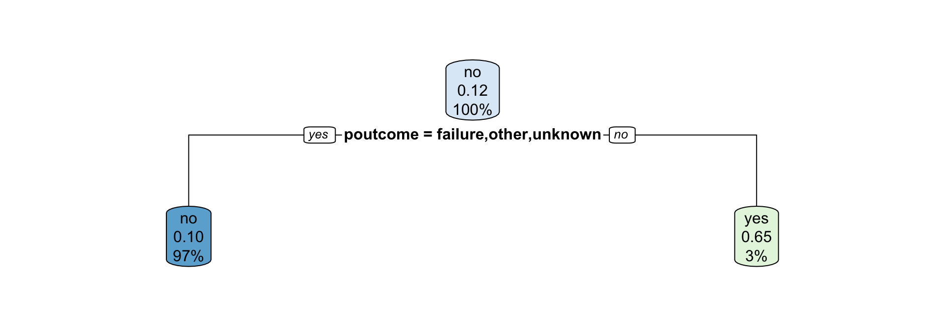
Partitions for categorical variables

When the variable is a categorical variable, the partition of observations is based on whether it belongs to a particular class or not.

E.g., there are 4 classes for poutcome and so 4 overall impurities are calculated, one for each class vs other.

Benefits of classification trees

The decision rules provided by trees are easy to explain and follow.
Trees search for optimal overall impurity independently for each predictor, therefore missing values in predictors can be better handled in trees.
Trees:
- can handle a mix of predictor types, categorical and quantitative,
- are robust to outliers,
- can capture non-linear relationships,
- invariant to transformations of predictors (as it is based on ordering).

Limitations of classification trees

Trees cannot model interaction between predictors.
The algorithm is greedy!
- This can result in a local optimal solution.
- It can often overfit the data (i.e. have high variance).
When separation is in linear combinations of variables trees struggle to provide a good classification.

Regression tree

Insurance cost

scroll

Recall this data sourced from the Medical Cost Personal Datasets in Week 2.

library(tidyverse)
insurance <- read_csv("https://emitanaka.org/iml/data/insurance.csv")
skimr::skim(insurance)

Data summary
Name	insurance
Number of rows	1338
Number of columns	7
_______________________
Column type frequency:
character	3
numeric	4
________________________
Group variables	None

Variable type: character

skim_variable	complete_rate	min	max	n_unique
sex	1	4	6	2
smoker	1	2	3	2
region	1	9	9	4

Variable type: numeric

skim_variable	complete_rate	mean	sd	p0	p25	p50	p75	p100	hist
age	1	39.21	14.05	18.00	27.00	39.00	51.00	64.00	▇▅▅▆▆
bmi	1	30.66	6.10	15.96	26.30	30.40	34.69	53.13	▂▇▇▂▁
children	1	1.09	1.21	0.00	0.00	1.00	2.00	5.00	▇▂▂▁▁
charges	1	13270.42	12110.01	1121.87	4740.29	9382.03	16639.91	63770.43	▇▂▁▁▁

Fitting regression tree with R

fit <- rpart(charges ~ ., data = insurance, method = "anova")
rpart.plot(fit)

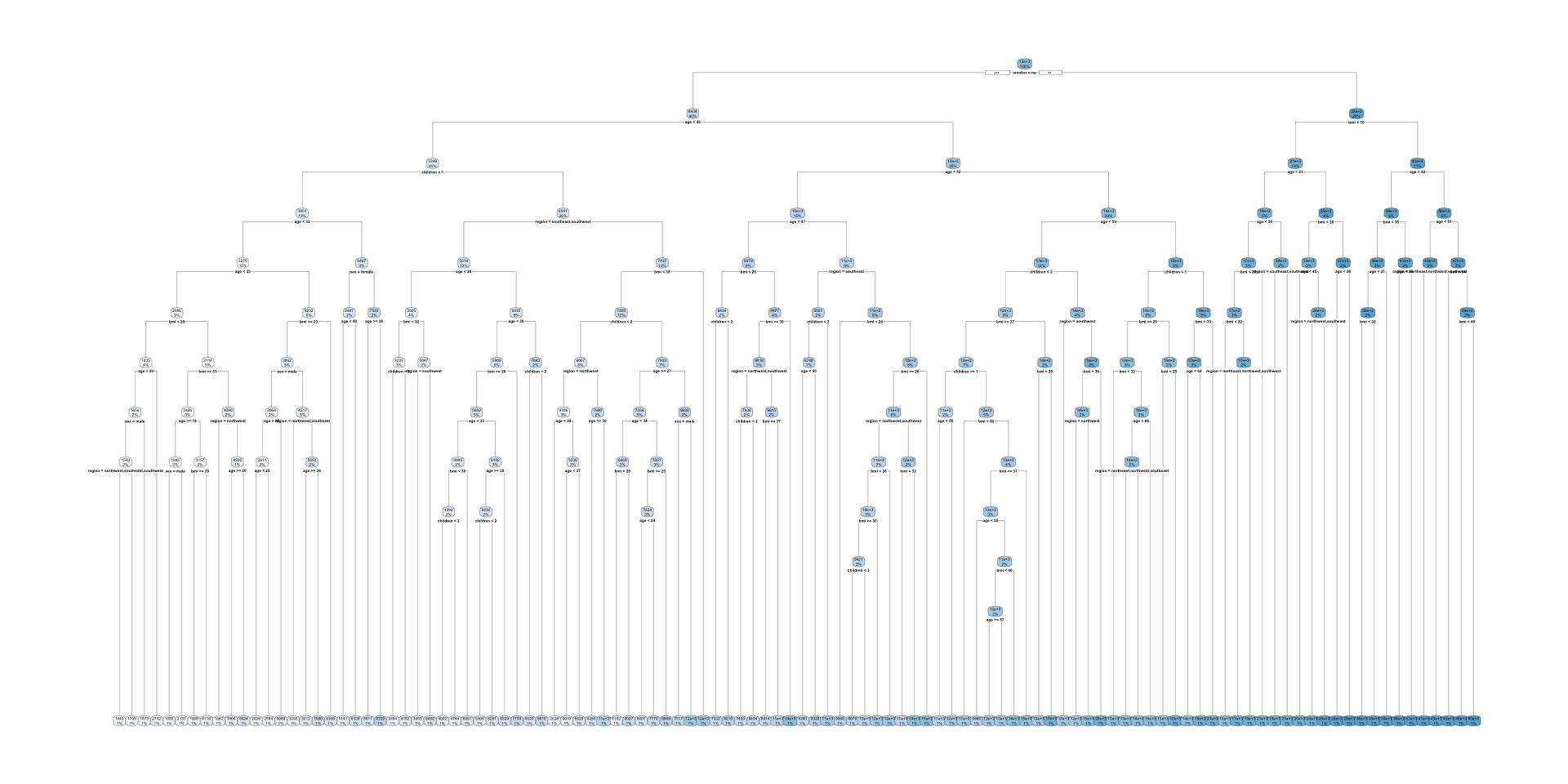
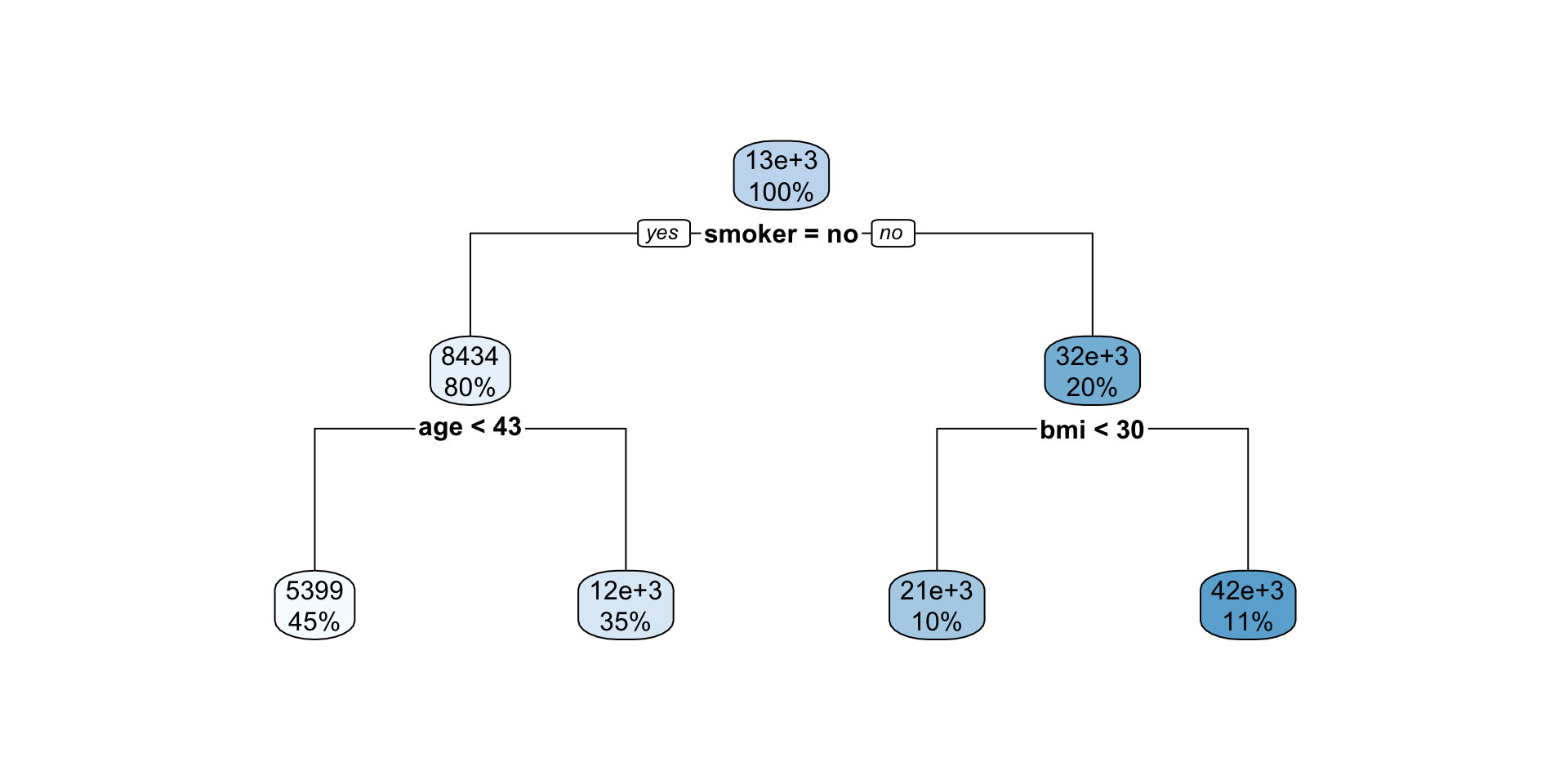
Interpreting regression tree plot

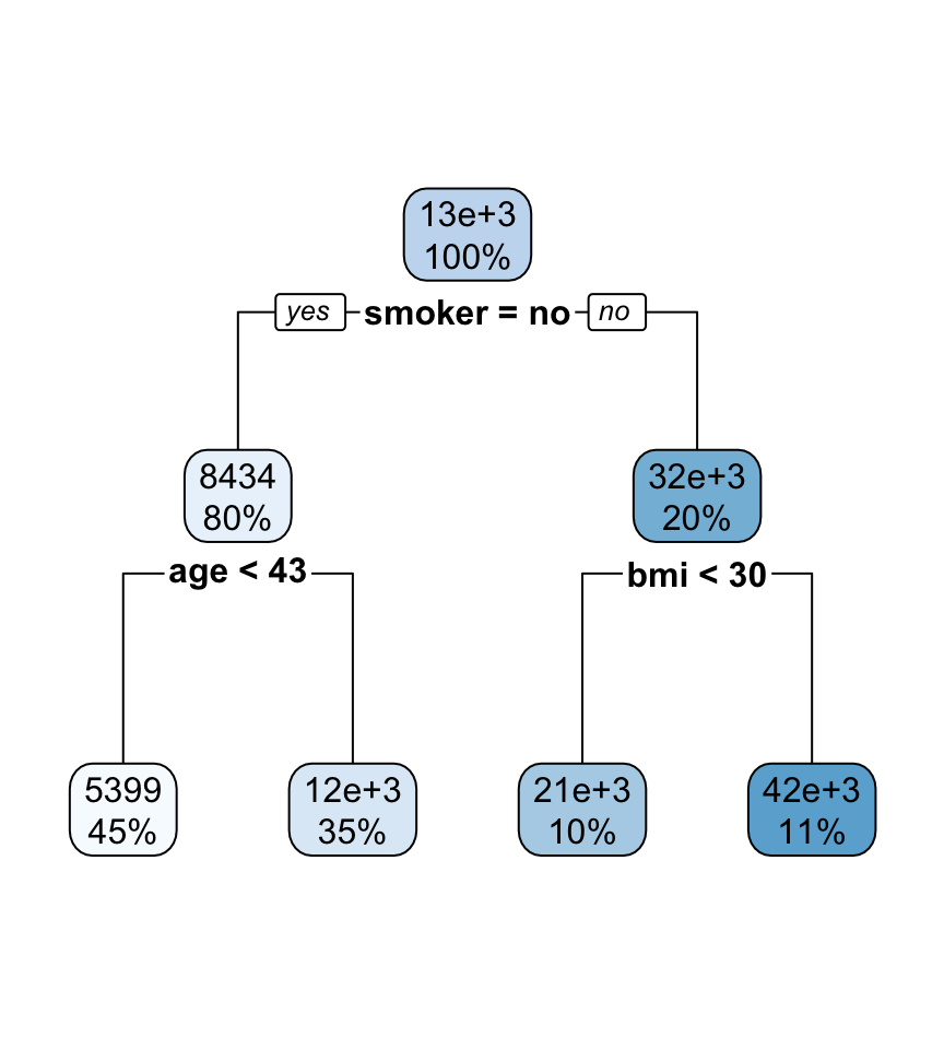
The nodes contain:
- average of the response, and
- percentage of observations in node.
The bold text shows the splitting rules (branches).
Colors indicate class, with a darker color indicating lower impurity.
The prediction is the average of the response in the terminal node.

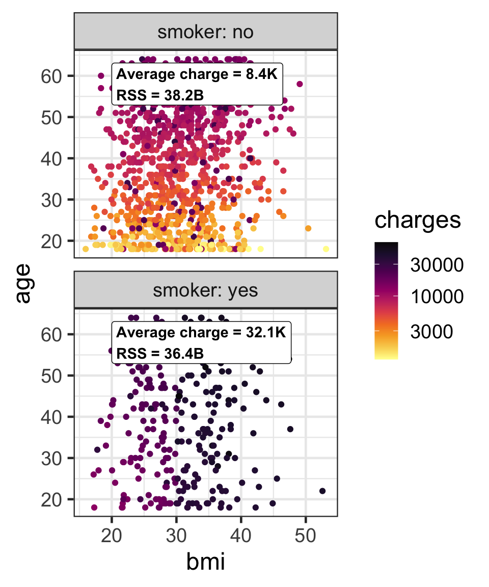
Partition based on a binary predictor

For a binary variable, \mathcal{A}_L and \mathcal{A}_R is based on its class.
Then find the average responses, \bar{y}_L and \bar{y}_R, for \mathcal{A}_L and \mathcal{A}_R, respectively.
We can use the residual sum of squares, e.g. \text{RSS}(\mathcal{A}_L) = \sum_{i \in \mathcal{A}_L}(y_i - \bar{y}_L)^2, to measure the impurity.
The overall impurity is \text{RSS}(\mathcal{A}_L) + \text{RSS}(\mathcal{A}_R) = 74.6\text{B}.

Partition based on a quantitative predictor

Like for classification trees, a quantitative predictor is partitioned based on the split value.
The overall impurity is based on a combined impurity measure for quantitative response (RSS here).

Pruning

We can grow a tree, T_0, and then prune it to a shorter tree (T_1).

T_0

T0 <- rpart(charges ~ ., 
            data = insurance, 
            method = "anova", 
            cp = 0)
rpart.plot(T0)

T_1

T1 <- prune(T0, cp = 0.01)
rpart.plot(T1)

Pruning to optimal `cp` based on `xerror`

scroll

We can select optimal cp based on xerror

T0$cptable %>% as_tibble()

# A tibble: 86 × 5
        CP nsplit `rel error` xerror   xstd
     <dbl>  <dbl>       <dbl>  <dbl>  <dbl>
 1 0.620        0       1      1.00  0.0519
 2 0.144        1       0.380  0.382 0.0190
 3 0.0637       2       0.236  0.239 0.0145
 4 0.00967      3       0.173  0.178 0.0133
 5 0.00784      4       0.163  0.172 0.0135
 6 0.00712      5       0.155  0.165 0.0131
 7 0.00537      6       0.148  0.157 0.0131
 8 0.00196      7       0.143  0.153 0.0132
 9 0.00190      8       0.141  0.156 0.0133
10 0.00173      9       0.139  0.154 0.0132
# ℹ 76 more rows

optimal_cp <- T0$cptable %>% 
              as.data.frame() %>% 
              filter(xerror == min(xerror)) %>% 
              # if multiple optimal points, then select one
              slice(1) %>% 
              pull(CP)
optimal_cp

[1] 0.0009125473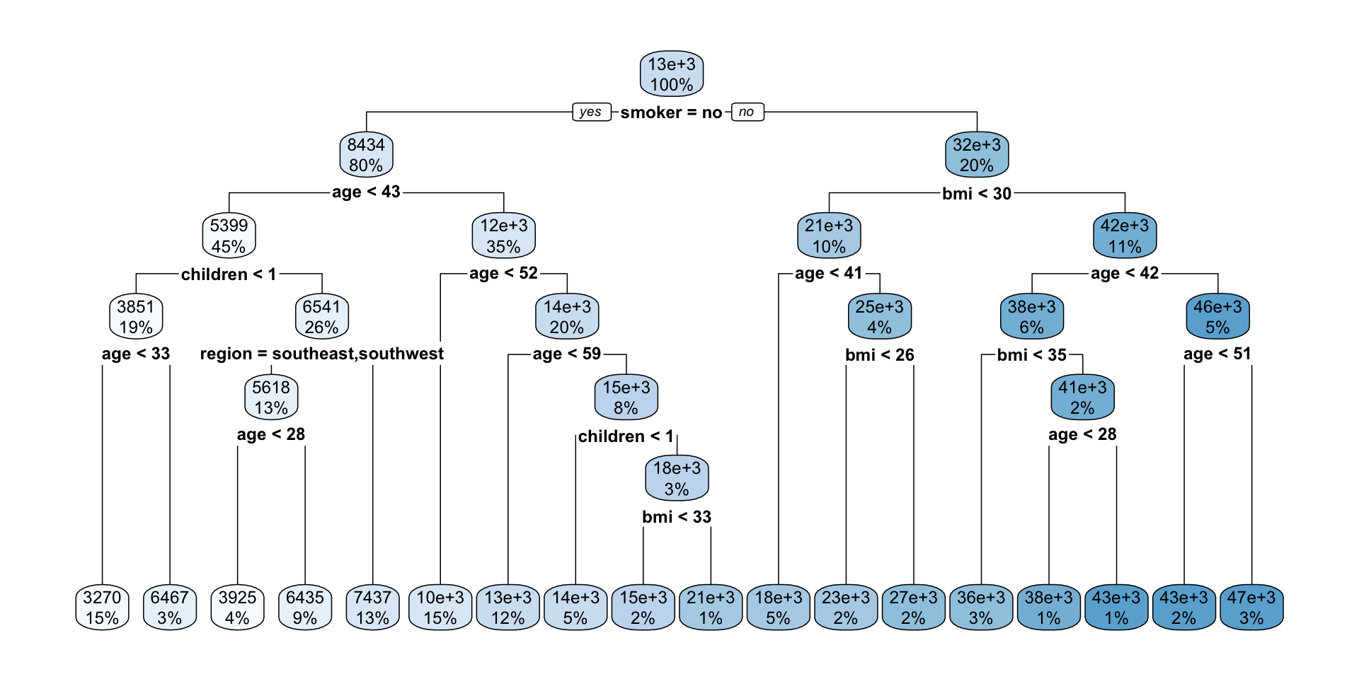

T2 <- prune(T0, cp = optimal_cp)
rpart.plot(T2)

Decision tree algorithm

Top-down: it begins at the top of the tree (all observations belong to a single region) and then successively splits the predictor space; each split is indicated via two new branches further down on the tree.
Greedy: at each step of the tree-building process, the best split is made at that particular step, rather than looking ahead and picking a split that will lead to a better tree in some future step.

Takeaway

Tree-based models consist of one or more of nested conditions for the predictors that partition the data.
Decision trees can be used for both regression and classification problems.
Decision trees used for:
- classification problems is referred to as classification trees, and
- regression problems is referred to as regression trees.

ETC3250/5250

Decision trees

Classification trees

Classification tree

Classification trees with R

Interpreting classification tree plot

Classifying new observations

Partition notation

Impurity metrics

Example calculation of Gini impurity index

Search for the optimal partition

Selected partition

Search for the next optimal partition

Stopping rules

Changing the stopping rules in rpart

Algorithm in a nutshell

Tuning parameters: search space

Tuning parameters: fit and predict

Tuning parameters: results

Tuning cp with cross validation error in rpart

Bank marketing data

Fitting and visualising the model

Partitions for categorical variables

Benefits of classification trees

Limitations of classification trees

Regression tree

Insurance cost

Fitting regression tree with R

Interpreting regression tree plot

Partition based on a binary predictor

Partition based on a quantitative predictor

Pruning

Pruning to optimal cp based on xerror

Decision tree algorithm

Takeaway

Changing the stopping rules in `rpart`

Tuning `cp` with cross validation error in `rpart`

Pruning to optimal `cp` based on `xerror`