Regularisation - table of contents

• 
  ETC3250/5250
  • Regularisation
• Too many predictors
• Ordinary least squares
• Visualising the RSS
• Shrinkage methods
• Ridge regression
  • Ridge regression
  • Shrinkage for ridge regression
  • Visualising the ridge regression constraint
  • Visualising the ridge regression
  • Lagrange function
  • Constrained vs unconstrained optimisation
  • Unconstrained optimization
  • Pre-processing data
  • Toyota car prices
  • Pre-processing data with recipes 📦
  • Pre-processed data with recipes 📦
  • Ridge regression in R
  • Regularisation path for ridge regression
  • Selecting the tuning parameter \(\lambda\)
  • Tuning parameter for ridge regression
  • Selecting the tuning parameter for ridge regression
  • Fitting the ridge regression model
  • A tidy, unified interface with tidymodels 📦
  • Limitation of ridge regression
• Lasso
  • Lasso
  • Visualising the lasso constraint
  • Visualising the lasso
  • Unconstrained representation for lasso
  • Lasso in R
  • Regularisation path for lasso
  • Selecting the tuning parameter \(\lambda\) for lasso
  • Lasso limitations
  • Group lasso
  • Group lasso in R
  • Regularisation path for group lasso
  • Regularisation path: lasso vs group lasso
  • Visualising the constraints
• Elastic net
  • Elastic net
• Takeaways

ETC3250/5250

Introduction to Machine Learning

Regularisation

Lecturer: Emi Tanaka

Department of Econometrics and Business Statistics

Too many predictors

• Subset selection methods are a useful way of selecting important predictors.
• However, they
  • are not guaranteed to provide the best model,
  • can be slow to compute if \(p\) is large, and
  • have issues when \(p > n\).
• Regularisation (shrinkage) methods avoid these issues.

Ordinary least squares

• OLS fits the coefficients as \[\hat{\boldsymbol\beta}= \underset{\boldsymbol\beta\in\mathbb{R}^{p+1}}{\mbox{arg min}}\ \sum_{i = 1}^n \left(y_i - \beta_0 - \sum_{j = 1}^p \beta_j x_{ij} \right)^2 = \underset{\boldsymbol\beta\in\mathbb{R}^{p+1}}{\mbox{arg min}}~\text{RSS}(\boldsymbol{\beta}).\]
• This is an unconstrained optimization problem.

Visualising the RSS

\[y_i = \beta_1x_{i1} + \beta_2x_{i2} + e_i,\]

• Data simulated with: \(\beta_1 = 2, \beta_2 = 3, e_i \sim N(0, 1)\)

• Axis grid

  • X: \(\beta_1\)
  • Y: \(\beta_2\)
  • Z: \(\text{RSS}(\beta_1, \beta_2)\)

Shrinkage methods

• Shrinkage methods fit a model containing all \(p\) predictors using a technique that constrains or regularizes the coefficient estimates.
• This shrinks some of the coefficient estimates towards zero.
• There are three main methods:
  • Ridge regression (also called L2 regularisation)
  • Lasso (also called L1 regularisation)
  • Elastic net (linear combination of L1 and L2 regularisation)

Ridge regression

Ridge regression

• Ridge regression is similar to except with constraint:

\[{\hat{\boldsymbol\beta}_{ridge} = \underset{\boldsymbol\beta\in\mathbb{R}^{p+1}}{\mbox{arg min}}\ \text{RSS}(\boldsymbol{\beta})} \color{#006DAE}{\quad {\text{subject to } \sum_{j=1}^p\beta_j^2\leq s}}.\]

• \(s\) bounds the magnitude of the coefficients.
• If \(s = 0\), then \(\beta_1, \dots, \beta_p\) are equal to zero.
• If \(s = \infty\), then ridge regression = OLS.

Shrinkage for ridge regression

\[\sum_{j=1}^p\beta_j^2\leq s\]

• Think of \(s\) as a budget - we allocate \(s\) to \(p\) predictors.
• Important predictors get a big part of the budget.
• In this formulation, \(\beta_j\) is shrunk towards zero (if the intercept is fitted into the model) but never actually zero.
• Shrinkage is not applied to the intercept coefficient.

Visualising the ridge regression constraint

• \(\beta_1^2 + \beta_2^2 \leq 1\)

• Axis grid

  • X: \(\beta_1\)
  • Y: \(\beta_2\)
  • Z: \(\text{RSS}(\beta_1, \beta_2)\)

Visualising the ridge regression

\[{\hat{\boldsymbol\beta} = \underset{\boldsymbol\beta\in\mathbb{R}^{2}}{\mbox{arg min}}\ \text{RSS}(\boldsymbol{\beta})}\]

\[\text{subject to } \beta_1^2 + \beta_2^2\leq s\]

• Axis grid
  • X: \(\beta_1\)
  • Y: \(\beta_2\)
  • Z: \(\text{RSS}(\beta_1, \beta_2)\)

Lagrange function

• Constrained optimization problems are much harder than unconstrained ones.

• Finding points in one surface is much easier than finding points simultaneously on both surfaces.

• Ridge regression can be re-written as a Lagrange function: \[\hat{\boldsymbol\beta}_{\text{ridge}} = \underset{\boldsymbol\beta\in\mathbb{R}^{p+1}}{\mbox{arg min}}~\left\{\text{RSS}(\boldsymbol{\beta}) + \lambda \sum_{j=1}^p \beta_j^2\right\}.\]

• \(\lambda \geq 0\) is called a tuning parameter and serves a similar role to \(s\).

• \(\lambda \sum_{j=1}^p \beta_j^2\) is referred to as the shrinkage penalty.

Constrained vs unconstrained optimisation

Constrained

Unconstrained

Unconstrained optimization

• This new problem has a closed form solution: \[\hat{\boldsymbol\beta}_{\text{ridge}} = (\mathbf{X}^\top\mathbf{X} + \lambda\mathbf{I}_{p + 1})^{-1}\mathbf{X}^\top\boldsymbol{y}\]
• Ridge regression will produce a different set of coefficients for each \(\lambda\).
• As \(\lambda\rightarrow\infty\), \(\hat{\beta}_1, \dots, \hat{\beta}_p\) will approach zero.
• If \(\lambda = 0\), ridge regression = OLS.
• \(\lambda\) is determined typically by cross-validation.

Pre-processing data

• Different measurement units of the predictors yields a different shrinkage penalty.
• This is an undesirable result and to avoid this, a common practice in ridge regression is to standardize (center and scale) the predictors.
• The standarisation of predictors may be done automatically for you in the software (read the documentation as always!).

Toyota car prices

library(tidyverse)
toyota <- read_csv("https://emitanaka.org/iml/data/toyota.csv")
glimpse(toyota)

Rows: 6,738
Columns: 9
$ model        <chr> "GT86", "GT86", "GT86", "GT86", "GT86", "GT86", "GT86", "…
$ year         <dbl> 2016, 2017, 2015, 2017, 2017, 2017, 2017, 2017, 2020, 201…
$ price        <dbl> 16000, 15995, 13998, 18998, 17498, 15998, 18522, 18995, 2…
$ transmission <chr> "Manual", "Manual", "Manual", "Manual", "Manual", "Manual…
$ mileage      <dbl> 24089, 18615, 27469, 14736, 36284, 26919, 10456, 12340, 5…
$ fuelType     <chr> "Petrol", "Petrol", "Petrol", "Petrol", "Petrol", "Petrol…
$ tax          <dbl> 265, 145, 265, 150, 145, 260, 145, 145, 150, 265, 265, 14…
$ mpg          <dbl> 36.2, 36.2, 36.2, 36.2, 36.2, 36.2, 36.2, 36.2, 33.2, 36.…
$ engineSize   <dbl> 2, 2, 2, 2, 2, 2, 2, 2, 2, 2, 2, 2, 2, 2, 2, 2, 2, 2, 2, …

Pre-processing data with recipes 📦

scroll

library(tidymodels)
library(rsample)
toyota_splits <- initial_split(toyota, prop = 0.75, strata = model)
toyota_recipe <- recipe(price ~ ., data = training(toyota_splits)) %>% 
  # standardising predictors
  step_normalize(all_numeric_predictors()) %>%  
  # change categorical variables to dummy variables
  step_dummy(all_nominal_predictors()) %>% 
  # remove any predictors with zero variance (i.e. constant)
  step_zv(all_predictors()) %>% 
  # log transform the response
  step_log(all_outcomes(), base = 10) %>% 
  # now signal that you are done
  prep()

toyota_recipe

Recipe

Inputs:

      role #variables
   outcome          1
 predictor          8

Training data contained 5052 data points and no missing data.

Operations:

Centering and scaling for year, mileage, tax, mpg, engineSize [trained]
Dummy variables from model, transmission, fuelType [trained]
Zero variance filter removed <none> [trained]
Log transformation on price [trained]

Pre-processed data with recipes 📦

toyota_train <- toyota_recipe %>% 
  bake(new_data = NULL)

toyota_test <- toyota_recipe %>% 
  bake(new_data = testing(toyota_splits))

toyota_test

# A tibble: 1,686 × 29
     year mileage   tax   mpg engineSize price model_A…¹ model…² model…³ model…⁴
    <dbl>   <dbl> <dbl> <dbl>      <dbl> <dbl>     <dbl>   <dbl>   <dbl>   <dbl>
 1 -0.342  0.0633 2.30  -1.72       1.20  4.20         0       0       0       0
 2 -0.798  0.241  2.30  -1.72       1.20  4.15         0       0       0       0
 3  0.114 -0.540  0.684 -1.72       1.20  4.26         0       0       0       0
 4  0.570  0.648  0.684 -1.72       1.20  4.27         0       0       0       0
 5  1.03  -1.06   0.752 -1.91       1.20  4.43         0       0       0       0
 6 -0.798  0.400  2.30  -1.72       1.20  4.15         0       0       0       0
 7  1.03  -1.02   0.684 -1.94       1.20  4.43         0       0       0       0
 8  0.570 -0.924  0.684 -1.72       1.20  4.32         0       0       0       0
 9 -1.71   1.45   2.30  -1.72       1.20  4.06         0       0       0       0
10  1.03  -1.20   0.684 -1.94       1.20  4.43         0       0       0       0
# … with 1,676 more rows, 19 more variables: model_Corolla <dbl>,
#   model_GT86 <dbl>, model_Hilux <dbl>, model_IQ <dbl>,
#   model_Land.Cruiser <dbl>, model_Prius <dbl>, model_PROACE.VERSO <dbl>,
#   model_RAV4 <dbl>, model_Supra <dbl>, model_Urban.Cruiser <dbl>,
#   model_Verso <dbl>, model_Verso.S <dbl>, model_Yaris <dbl>,
#   transmission_Manual <dbl>, transmission_Other <dbl>,
#   transmission_Semi.Auto <dbl>, fuelType_Hybrid <dbl>, …

Ridge regression in R

• Ridge regression for a particular \(\lambda\) can be fit using the glmnet package.

library(glmnet)
# namespace conflict with MASS::select, so this needs to be overwritten
select <- dplyr::select 

lambda_vec <- 10^seq(-10, 0, length = 50)
fit_ridge <- glmnet(x = toyota_train %>% 
                     select(-price),
                    y = toyota_train$price,
                    alpha = 0, # we'll explain this later
                    lambda = lambda_vec)

• Note: the glmnet package doesn’t use symbolic model formula and requires categorical variables to be converted to dummy variables.

Regularisation path for ridge regression

Code

library(broom) # for tidy
fit_ridge %>% 
  tidy(return_zeros = TRUE) %>% 
  filter(term != "(Intercept)") %>%  
  ggplot(aes(lambda, estimate))  +
  geom_line(data = ~rename(., term2 = term), 
            aes(group = term2),
            color = "grey") + 
  geom_hline(yintercept = 0, linetype = "dashed") +
  geom_line(color = "royalblue2") + 
  facet_wrap(~term, nrow = 4) +
  labs(x = latex2exp::TeX("\\lambda"),
       y = "Standardised coefficients") +
  scale_x_log10()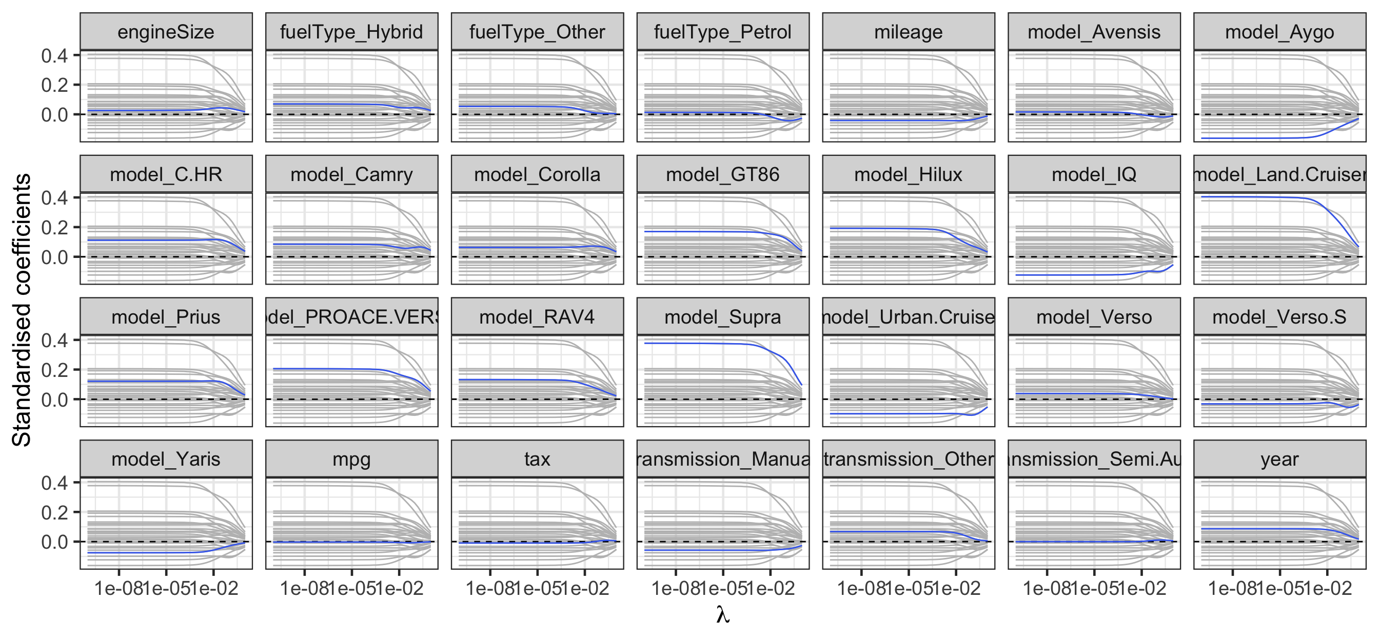

Selecting the tuning parameter \(\lambda\)

scroll

cv_glmnet_to_toyota <- function(alpha) {
  # Note: you're applying cross validation to the training dataset!
  toyota_train %>% 
    # make the 10-fold cross validation data set
    vfold_cv(v = 10) %>% 
    # for each fold, calculate the model metrics
    mutate(metrics = map(splits, function(.split) {
      # get the fold training dataset
      fold_train_data <- training(.split)
    
      # fit the model to the fold training dataset
      fold_fit <- glmnet(x = fold_train_data %>% 
                                        select(-price),
                         y = fold_train_data$price,
                         alpha = alpha,
                         lambda = lambda_vec)
        
      # now get the validation dataset
      fold_test_data <- testing(.split)
    
      # get the predictions for this fold and models
      fold_preds <- fold_fit %>% 
          predict(as.matrix(select(fold_test_data, -price))) %>% 
          as.data.frame() %>% 
          add_column(price = fold_test_data$price) %>% 
          pivot_longer(-price, values_to = ".pred", names_to = "name") %>% 
          left_join(tibble(name = paste0("s", 1:length(lambda_vec) - 1), 
                           lambda = rev(lambda_vec)),
                    by = "name")
        
      # get the model metrics for this fold
      fold_preds %>% 
          group_by(name, lambda) %>% 
          metric_set(rmse, mae, mape)(., price, .pred) %>% 
          select(-.estimator) %>% 
          arrange(.metric, lambda)
    
  })) %>% 
  # summarise the model metrics for each value of lambda
  unnest(metrics) %>% 
  group_by(name, .metric) %>% 
  summarise(lambda = unique(lambda), 
            mean = mean(.estimate), 
            se = sd(.estimate))
}

Tuning parameter for ridge regression

toyota_tuning_ridge  <- cv_glmnet_to_toyota(alpha = 0)

toyota_tuning_ridge

# A tibble: 150 × 5
# Groups:   name [50]
   name  .metric  lambda   mean      se
   <chr> <chr>     <dbl>  <dbl>   <dbl>
 1 s0    mae     1       0.104  0.00353
 2 s0    mape    1       2.59   0.0903 
 3 s0    rmse    1       0.140  0.00490
 4 s1    mae     0.625   0.0891 0.00292
 5 s1    mape    0.625   2.22   0.0757 
 6 s1    rmse    0.625   0.121  0.00451
 7 s10   mae     0.00910 0.0327 0.00130
 8 s10   mape    0.00910 0.817  0.0360 
 9 s10   rmse    0.00910 0.0454 0.00366
10 s11   mae     0.00569 0.0325 0.00132
# … with 140 more rows

Selecting the tuning parameter for ridge regression

Code

toyota_tuning_ridge_min <- toyota_tuning_ridge %>% 
               group_by(.metric) %>% 
               filter(mean == min(mean))


toyota_tuning_ridge %>% 
  ggplot(aes(lambda, mean)) +
  geom_errorbar(aes(ymin = mean - se,
                    ymax = mean + se)) +
  geom_line() +
  geom_point(data = toyota_tuning_ridge_min,
             color = 'red') +
  facet_wrap(~.metric, scales = "free") +
  scale_x_log10(name = latex2exp::TeX("\\lambda"))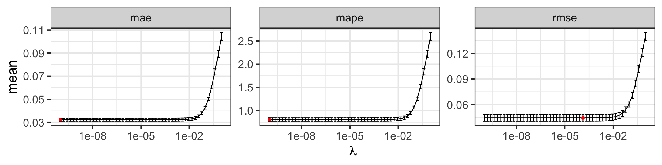

Metric	\(\lambda\)	Mean	Std. Error
rmse	0.0001326	0.0445490	0.0039625
mae	0.0000000	0.0322999	0.0013496
mape	0.0000000	0.8054924	0.0367295

Fitting the ridge regression model

best_lambda_ridge <- toyota_tuning_ridge_min$lambda[1]

fit_ridge <- glmnet(x = toyota_train %>%
                      select(-price),
                    y = toyota_train$price,
                    alpha = 0,
                    lambda = best_lambda_ridge)

• Even though the context of this machine learning is linear regression, the interface for glmnet is different to lm that used a symbolic model formula.
• Ideally these interfaces are standardised, but as methods are developed often by independent parties, differences often arise.
• It is important that you learn to make use of documentation and fit toy models to understand what functions are doing.

A tidy, unified interface with tidymodels 📦

• parsnip (part of tidymodels) standardises this interface.

workflow(toyota_recipe) %>% 
  add_model(linear_reg(engine = "glmnet", penalty = best_lambda_ridge, mixture = 0)) %>% 
  fit(testing(toyota_splits)) %>% 
  tidy()

# A tibble: 27 × 3
   term          estimate  penalty
   <chr>            <dbl>    <dbl>
 1 (Intercept)    4.11    0.000133
 2 year           0.0827  0.000133
 3 mileage       -0.0463  0.000133
 4 tax           -0.00728 0.000133
 5 mpg           -0.00608 0.000133
 6 engineSize     0.0369  0.000133
 7 model_Avensis -0.0310  0.000133
 8 model_Aygo    -0.129   0.000133
 9 model_C.HR     0.115   0.000133
10 model_Camry    0.0283  0.000133
# … with 17 more rows

Limitation of ridge regression

• It will always use all \(p\) predictors!
• While it shrinks coefficients towards zero, it does not set it exactly to zero.
• Lasso is an alternative approach that induces a sparse model.

Lasso

Lasso

• Least absolute shrinkage and selection operator (lasso) is similar to ridge regression except for the constraint of the optimization problem:

\[{\hat{\boldsymbol\beta}_{lasso} = \underset{\boldsymbol\beta\in\mathbb{R}^{p+1}}{\mbox{arg min}}\ \text{RSS}(\boldsymbol{\beta})}\quad \color{#006DAE}{\text{subject to } \sum_{j=1}^p|\beta_j|\le s}.\]

Visualising the lasso constraint

• \(s\) bounds the magnitude of the coefficients.
• If \(s = 0\), all betas are equal to zero.
• If \(s = \infty\), then the LASSO = OLS.
• Axis grid:
  • X: \(\beta_1\)
  • Y: \(\beta_2\)

Visualising the lasso

• For LASSO, \(\hat{\beta}_2 = 0\)!
• LASSO produces sparse models.
• Axis grid:
  • X: \(\beta_1\)
  • Y: \(\beta_2\)
  • Z: \(\text{RSS}(\beta_1, \beta_2)\)

Unconstrained representation for lasso

\[\hat{\boldsymbol\beta} = \underset{\boldsymbol\beta\in\mathbb{R}^{p+1}}{\mbox{arg min}}\left\{~\text{RSS}(\boldsymbol{\beta}) + \underbrace{\lambda \sum_{j=1}^p |\beta_j|}_{\large\text{shrinkage penalty}}\right\}\]

• \(\lambda \geq 0\) is a tuning parameter.
• Larger \(\lambda\) more shrinkage, smaller \(\lambda\) less shrinkage.
• \(\lambda\) can be chosen again via cross-validation.

Lasso in R

• Lasso for a particular \(\lambda\) can also be fit using the glmnet package.

fit_lasso <- glmnet(x = toyota_train %>% 
                     select(-price),
                    y = toyota_train$price,
                    alpha = 1,
                    lambda = lambda_vec)

• Note here that the alpha = 1 (again, we’ll explain why later).

Regularisation path for lasso

Code

library(broom) # for tidy
est_lasso <- fit_lasso %>% 
  tidy(return_zeros = TRUE)

est_lasso %>% 
  filter(term != "(Intercept)") %>%  
  mutate(zero = estimate == 0) %>% 
  ggplot(aes(lambda, estimate))  +
  geom_line(data = ~rename(., term2 = term), 
            aes(group = term2),
            color = "grey") + 
  geom_hline(yintercept = 0, linetype = "dashed") +
  geom_line(aes(color = zero, group = term)) + 
  facet_wrap(~term, nrow = 4) +
  labs(x = latex2exp::TeX("\\lambda"),
       y = "Standardised coefficients") +
  guides(color = "none") +
  scale_x_log10()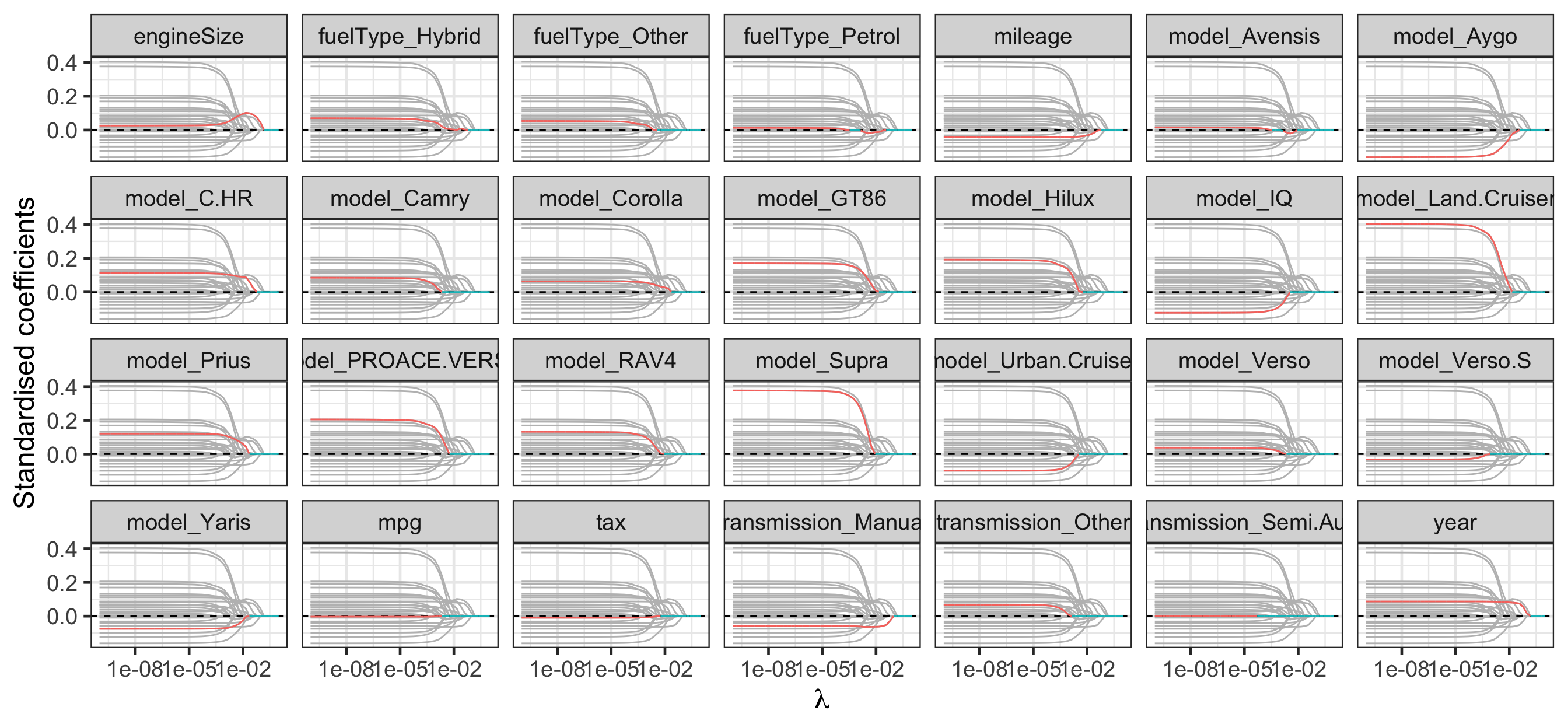

Selecting the tuning parameter \(\lambda\) for lasso

Code

toyota_tuning_lasso <- cv_glmnet_to_toyota(alpha = 1)

toyota_tuning_lasso_min <- toyota_tuning_lasso %>% 
  group_by(.metric) %>% 
  filter(mean == min(mean))

toyota_tuning_lasso %>% 
  ggplot(aes(lambda, mean)) +
  geom_errorbar(aes(ymin = mean - se,
                    ymax = mean + se)) +
  geom_line() +
  geom_point(data = toyota_tuning_lasso_min, 
             color = 'red') +
  facet_wrap(~.metric, scales = "free") +
  scale_x_log10(name = latex2exp::TeX("\\lambda"))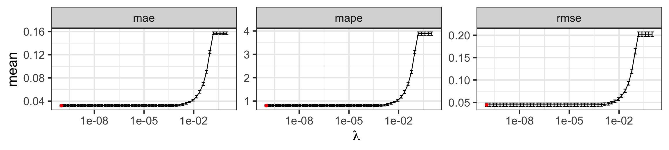 

Metric	\(\lambda\)	Mean	Std. Error
mae	0	0.0323048	0.0017061
mape	0	0.8057043	0.0447169
rmse	0	0.0446230	0.0039084

Lasso limitations

• If a group of predictors are highly correlated, lasso will pick one of them at random, which is not desirable!

• There may be a grouping structure amongst the variables (e.g. dummy variables that belong to the same categorical variable) – in lasso, grouped variables are not simultaneously zero, which can result in only a subset of levels of a categorical variable being selected.

Group lasso

• We can change the penalty to induce a group sparsity.

\[\hat{\boldsymbol\beta}_{glasso} = \underset{\boldsymbol\beta\in\mathbb{R}^{p+1}}{\mbox{arg min}}\left\{~\text{RSS}(\boldsymbol{\beta}) + \lambda \sum_{j}||\boldsymbol{\beta}_j||\right\}\]

• \(\boldsymbol{\beta}_j\) denotes the vector of regression coefficients corresponding to the \(j\)-th group.
• \(\beta_{jk}\) denotes the \(k\)-th regression coefficient in the \(j\)-th group.
• \(||\boldsymbol{\beta}_j||\) denotes the Euclidean (\(L_2\)) norm of \(\boldsymbol{\beta}_j\).

Group lasso in R

• Group lasso for a particular \(\lambda\) can be fit using the grpreg package.

library(grpreg)
groups <- str_replace(names(toyota_train %>% select(-price)), "_.+", "")
groups 

 [1] "year"         "mileage"      "tax"          "mpg"          "engineSize"  
 [6] "model"        "model"        "model"        "model"        "model"       
[11] "model"        "model"        "model"        "model"        "model"       
[16] "model"        "model"        "model"        "model"        "model"       
[21] "model"        "model"        "transmission" "transmission" "transmission"
[26] "fuelType"     "fuelType"     "fuelType"    

fit_glasso <- grpreg(X = toyota_train %>% 
                        select(-price),
                     y = toyota_train$price,
                     group = groups,
                     alpha = 1,
                     penalty = "grLasso",
                     lambda = lambda_vec)

Regularisation path for group lasso

Code

est_glasso <- fit_glasso %>% 
  broom:::tidy.glmnet(return_zeros = TRUE)

est_glasso %>% 
  mutate(zero = estimate == 0) %>% 
  filter(term != "(Intercept)") %>%  
  ggplot(aes(lambda, estimate))  +
  geom_line(data = ~rename(., term2 = term), 
            aes(group = term2),
            color = "grey") + 
  geom_hline(yintercept = 0, linetype = "dashed") +
  geom_line(aes(color = zero, group = term)) + 
  facet_wrap(~term, nrow = 4) +
  labs(x = latex2exp::TeX("\\lambda"),
       y = "Standardised coefficients") +
  scale_x_log10() +
  guides(color = "none")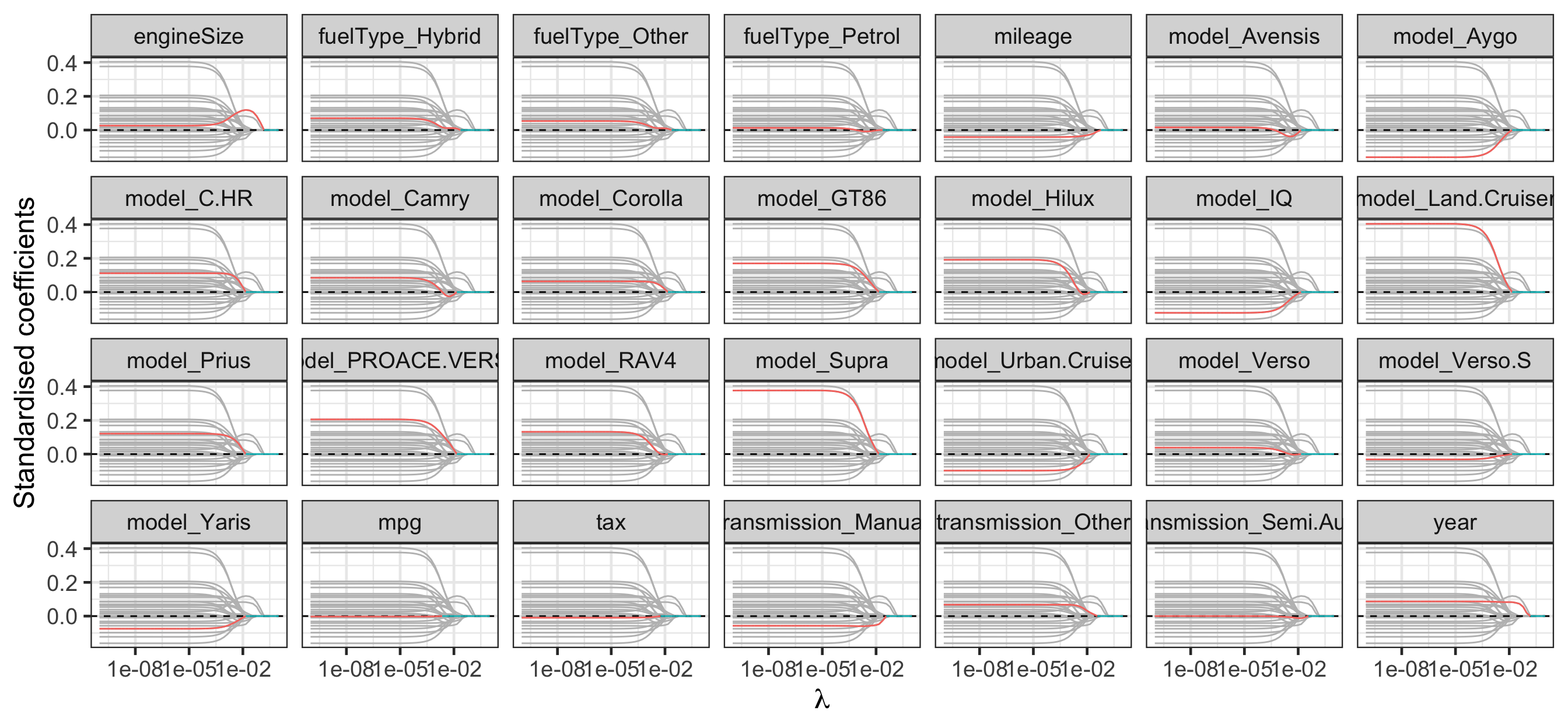

Regularisation path: lasso vs group lasso

scroll

Code

bind_rows(mutate(est_lasso, type = "lasso"),
          mutate(est_glasso, type = "glasso")) %>% 
  mutate(type = fct_inorder(type), 
         zero = estimate == 0) %>% 
  filter(str_detect(term, "^(model_|transmission_)")) %>%  
  ggplot(aes(lambda, estimate))  +
  geom_hline(yintercept = 0, linetype = "dashed") +
  geom_line(aes(group = interaction(term, type), color = type)) + 
  facet_wrap(~term) + 
  labs(x = latex2exp::TeX("\\lambda"),
       y = "Standardised coefficients") +
  scale_x_log10() +
  scale_color_manual("", values = c("royalblue2", "violetred2"))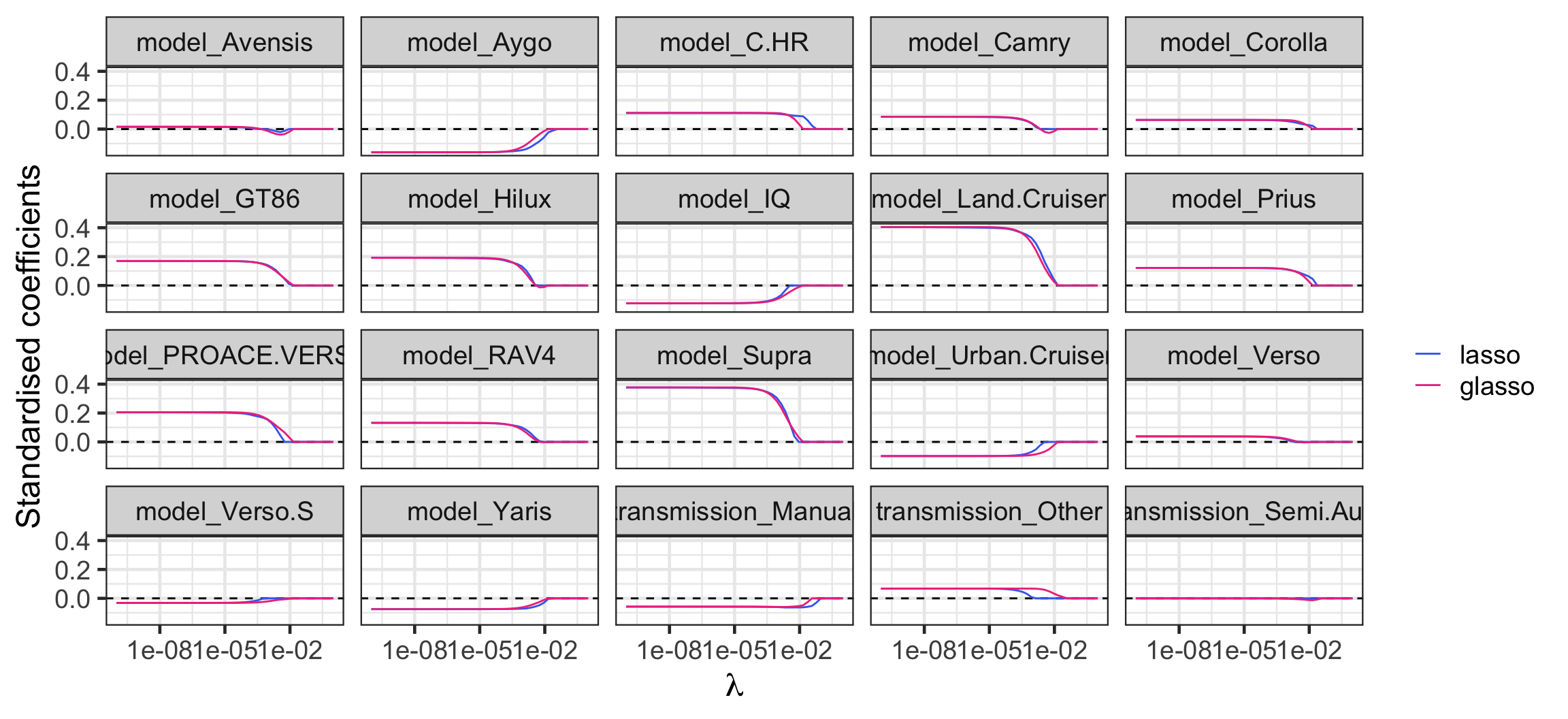

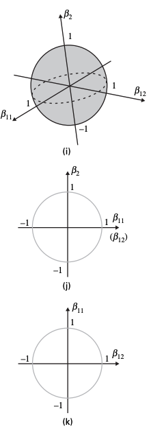
Visualising the constraints

Lasso

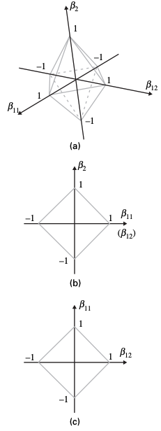
Group lasso

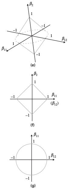
Ridge regression

Figures from Yuan & Lin (2006) Model selection and estimation in regression with grouped variables

Elastic net

Elastic net

• Elastic net is an approach that combines LASSO and ridge regression.

\[\hat{\boldsymbol\beta}_{elastic} = \underset{\boldsymbol\beta\in\mathbb{R}^{p+1}}{\mbox{arg min}}\ \left\{\text{RSS}(\boldsymbol{\beta})+\lambda\left(\frac{1-\alpha}{2}\sum_{j=1}^p\beta_j^2+\alpha\sum_{j=1}^p|\beta_j|\right)\right\}.\]

• \(\alpha\) is another tuning parameter.
• If \(\alpha = 1\), elastic net = lasso.
• If \(\alpha = 0\), elastic net = ridge regression.
• You can pick \(\lambda\) and \(\alpha\) via cross-validation.

Takeaways

• Shrinkage methods are a powerful variable selection approach for regression by shrinking the coefficients predictors towards zero.
• You can use cross-validation to calibrate these methods for prediction.