ETC3250/5250

Introduction to Machine Learning

Resampling

Lecturer: Emi Tanaka

Department of Econometrics and Business Statistics

Resampling

Resampling is a process of making new data based on observed data.
Commonly used resampling methods include:
- Cross validation
  - often used for model assessment.
- Bootstrapping
  - often used to provide a measure of accuracy of a parameter estimate.

Recall: training, validation and testing data sets

In Lecture 1, randomly splitting 75% of data into training data and the remaining 25% into testing data, then measured the accuracy of model trained on the training data using the testing data.
But the model accuracy changes on a different split.
Cross-validation extends this approach to:
- several iterations of different splits, and
- combine (typically by averaging) the model accuracy across the iterations.

Cross validation

\(k\)-fold cross validation

Partition samples into \(k\) (near) equal sized subsamples (referred to as folds).
Fit the model on \(k − 1\) subsets, and compute a metric, e.g. RMSE, on the omitted subset.
Repeat \(k\) times omitting a different subset each time.

Cross validation accuracy

Choice of \(k = 10\) is common.
Recall from Lecture 1 there are a number of ways to measure preditive accuracy, e.g. RMSE, MAE, MAPE and MPE.
Cross-validation accuracy is calculated:
- by calculating the accuracy (based on one metric) on every fold, then
- combining this into a single number, e.g. by taking a simple average.

\(k\)-fold cross validation with `rsample`

\(k = 5\) fold cross validation (\(k =\) v in the rsample package)

library(tidyverse)
library(rsample)
toyota <- read_csv("https://emitanaka.org/iml/data/toyota.csv") 
set.seed(2023) # to replicate result
toyota_folds <- vfold_cv(toyota, v = 5) 
toyota_folds

#  5-fold cross-validation 
# A tibble: 5 × 2
  splits              id   
  <list>              <chr>
1 <split [5390/1348]> Fold1
2 <split [5390/1348]> Fold2
3 <split [5390/1348]> Fold3
4 <split [5391/1347]> Fold4
5 <split [5391/1347]> Fold5

Measuring accuracy for a single fold

scroll

Each fold is an rsplit object:

toyota_folds$splits[[1]]

<Analysis/Assess/Total>
<5390/1348/6738>

So you can extract the training and testing data as before:

toyota_train1 <- training(toyota_folds$splits[[1]])
toyota_test1 <- testing(toyota_folds$splits[[1]])

And train models as before:

library(rpart) # for regression tree
library(kknn) # for k-nearest neighbour
model_fits <- list(
  "reg" = lm(log10(price) ~ year,
             data = toyota_train1),
  "tree" = rpart(log10(price) ~ year,
                 data = toyota_train1,
                 method = "anova"),
  "knn" = train.kknn(log10(price) ~ year,
                     data = toyota_train1)
)

Then predict responses:

results_test1 <- imap_dfr(model_fits, ~{
    toyota_test1 %>% 
      select(year, price) %>% 
      mutate(.model = .y,
             .pred = 10^predict(.x, .))
  })

and finally measure predictive accuracy for this fold:

library(yardstick)
results_test1 %>% 
  group_by(.model) %>% 
  metric_set(rmse, mae, mape, mpe, rsq)(., price, .pred) %>% 
  pivot_wider(.model, names_from = .metric, values_from = .estimate)

# A tibble: 3 × 6
  .model  rmse   mae  mape    mpe   rsq
  <chr>  <dbl> <dbl> <dbl>  <dbl> <dbl>
1 knn    7808. 6631.  70.4 -64.7  0.188
2 reg    5364. 4123.  33.7  -8.23 0.186
3 tree   5380. 4121.  33.8  -8.67 0.178

Fitting the models for each fold

toyota_models <- toyota_folds %>% 
  # fit models 
  mutate(reg = map(splits, ~lm(log10(price) ~ year, data = training(.x))),
         tree = map(splits, ~rpart(log10(price) ~ year, data = training(.x), method = "anova")),
         knn = map(splits, ~train.kknn(log10(price) ~ year, data = training(.x))))

toyota_models

#  5-fold cross-validation 
# A tibble: 5 × 5
  splits              id    reg    tree    knn       
  <list>              <chr> <list> <list>  <list>    
1 <split [5390/1348]> Fold1 <lm>   <rpart> <trn.kknn>
2 <split [5390/1348]> Fold2 <lm>   <rpart> <trn.kknn>
3 <split [5390/1348]> Fold3 <lm>   <rpart> <trn.kknn>
4 <split [5391/1347]> Fold4 <lm>   <rpart> <trn.kknn>
5 <split [5391/1347]> Fold5 <lm>   <rpart> <trn.kknn>

Measuring accuracy for each fold

scroll

toyota_metrics <- toyota_models %>% 
  mutate(across(c(reg, tree, knn), function(models) {
    # now for every fold and model, 
    map2(splits, models, function(.split, .model) {
      testing(.split) %>% 
        # compute prediction for testing set
        mutate(.pred = 10^predict(.model, .)) %>% 
        # then get metrics
        metric_set(rmse, mae, mape, mpe, rsq)(., price, .pred) %>%  
        # in a one-row data frame such that 
        # column names are metric, 
        # values are the accuracy measure
        pivot_wider(-.estimator,
                    names_from = .metric, 
                    values_from = .estimate)
    })
  }, .names = "{.col}_metrics"))

toyota_metrics

#  5-fold cross-validation 
# A tibble: 5 × 8
  splits              id    reg    tree    knn        reg_metrics     
  <list>              <chr> <list> <list>  <list>     <list>          
1 <split [5390/1348]> Fold1 <lm>   <rpart> <trn.kknn> <tibble [1 × 5]>
2 <split [5390/1348]> Fold2 <lm>   <rpart> <trn.kknn> <tibble [1 × 5]>
3 <split [5390/1348]> Fold3 <lm>   <rpart> <trn.kknn> <tibble [1 × 5]>
4 <split [5391/1347]> Fold4 <lm>   <rpart> <trn.kknn> <tibble [1 × 5]>
5 <split [5391/1347]> Fold5 <lm>   <rpart> <trn.kknn> <tibble [1 × 5]>
  tree_metrics     knn_metrics     
  <list>           <list>          
1 <tibble [1 × 5]> <tibble [1 × 5]>
2 <tibble [1 × 5]> <tibble [1 × 5]>
3 <tibble [1 × 5]> <tibble [1 × 5]>
4 <tibble [1 × 5]> <tibble [1 × 5]>
5 <tibble [1 × 5]> <tibble [1 × 5]>

toyota_metrics$reg_metrics[[1]]

# A tibble: 1 × 5
   rmse   mae  mape   mpe   rsq
  <dbl> <dbl> <dbl> <dbl> <dbl>
1 5364. 4123.  33.7 -8.23 0.186

Examining the fold results

toyota_metrics_wide <- toyota_metrics %>% 
  # expand to see results
  unnest_wider(ends_with("_metrics"), names_sep = "_") %>% 
  # wrangle data into output form below
  pivot_longer(contains("metrics"), 
               names_to = c("model", "metric"),
               names_pattern = "(.*)_metrics_(.*)",
               values_to = "value") %>% 
  pivot_wider(c(id, model),
              names_from = metric,
              values_from = value) 

toyota_metrics_wide

# A tibble: 15 × 7
   id    model  rmse   mae  mape    mpe   rsq
   <chr> <chr> <dbl> <dbl> <dbl>  <dbl> <dbl>
 1 Fold1 reg   5364. 4123.  33.7  -8.23 0.186
 2 Fold1 tree  5380. 4121.  33.8  -8.67 0.178
 3 Fold1 knn   7808. 6631.  70.4 -64.7  0.188
 4 Fold2 reg   5633. 4227.  33.6  -6.62 0.193
 5 Fold2 tree  5585. 4184.  33.4  -6.45 0.207
 6 Fold2 knn   7508. 6285.  65.2 -57.6  0.205
 7 Fold3 reg   5845. 4240.  34.5  -7.94 0.245
 8 Fold3 tree  5794. 4197.  34.9  -8.42 0.262
 9 Fold3 knn   8880. 7337.  78.0 -71.7  0.192
10 Fold4 reg   6010. 4200.  33.3  -7.79 0.184
11 Fold4 tree  5964. 4149.  33.0  -7.93 0.196
12 Fold4 knn   8512. 7092.  73.8 -68.9  0.192
13 Fold5 reg   5984. 4273.  33.3  -6.84 0.195
14 Fold5 tree  5949. 4219.  33.0  -7.00 0.201
15 Fold5 knn   7902. 6602.  68.9 -63.3  0.207

Getting the cross validation metrics

toyota_metrics_wide %>% 
  # get the average of each metric columns
  group_by(model) %>% 
  summarise(across(rmse:rsq, mean))

# A tibble: 3 × 6
  model  rmse   mae  mape    mpe   rsq
  <chr> <dbl> <dbl> <dbl>  <dbl> <dbl>
1 knn   8122. 6790.  71.3 -65.2  0.197
2 reg   5767. 4212.  33.7  -7.48 0.201
3 tree  5734. 4174.  33.6  -7.69 0.209

But a numerical summary alone can be deceiving in understand what is the best model.

Visualising with parallel coordinate plots

toyota_metrics_wide %>% 
  GGally::ggparcoord(columns = 3:7,
                     groupColumn = 2,
                     showPoints = TRUE) +
  labs(x = "metric")

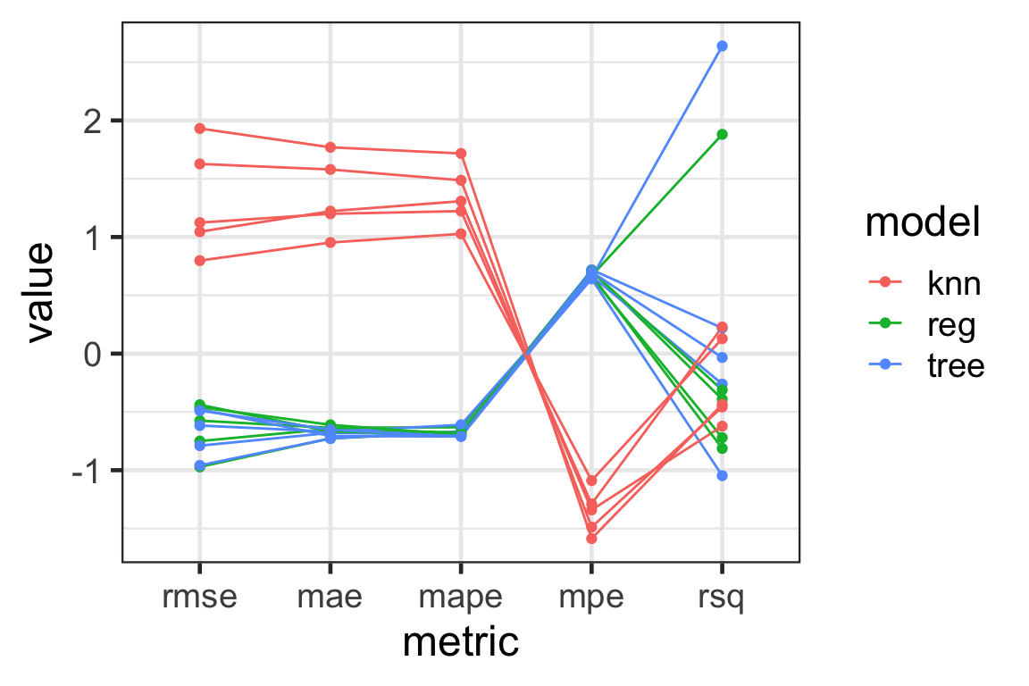
Parallel coordinate plots can be used to visualise high-dimensional data - here our model metrics!
Each variable is shown in the \(x\)-axis.
The value of the variable is standardised in this plot.
The lines correspond to an observational unit (a fold and a model combination).
The lines are colored by the model here.

Results

We see that knn has a large variation in the metrics - this means this model has a high variance and it is not desirable.
The tree and reg has a large variation in rmse and rsq - they are somewhat similar in performance.

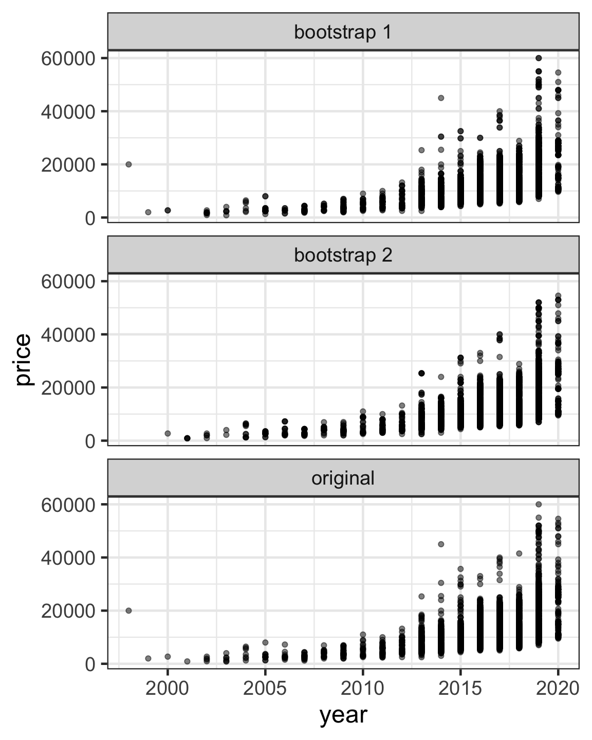
Leave-one-out cross validation (LOOCV)

LOOCV is a special case of \(k\)-fold cross validation where \(k = n\) (or \(n_{Train}\)).

toyota %>% 
  vfold_cv(v = n())

The rsample package has a specific function for this special case that is essentially similar to above:

toyota %>% 
  loo_cv()

# Leave-one-out cross-validation 
# A tibble: 6,738 × 2
   splits           id        
   <list>           <chr>     
 1 <split [6737/1]> Resample1 
 2 <split [6737/1]> Resample2 
 3 <split [6737/1]> Resample3 
 4 <split [6737/1]> Resample4 
 5 <split [6737/1]> Resample5 
 6 <split [6737/1]> Resample6 
 7 <split [6737/1]> Resample7 
 8 <split [6737/1]> Resample8 
 9 <split [6737/1]> Resample9 
10 <split [6737/1]> Resample10
# … with 6,728 more rows

Bias-variance tradeoff for cross validation

\(k\)-fold cross validation with \(k < n\) has a computational advantage over LOOCV (\(k = n\)).
LOOCV is preferred to \(k\)-fold cross validation in the perspective of bias reduction (almost all data are used to estimate the model).
\(k\)-fold cross validation is preferred to LOOCV in the perspective of lower variance (the \(n\) fitted models in LOOCV are going to be highly positively correlated).
We usually select \(k=5\) or \(k=10\) to balance the bias-variance trade-off.

Bootstrap

Bootstrap samples

A bootstrap sample is created by sampling with replacement the original data with the same dimension as the original data.

set.seed(2023) # to replicate results
toyota %>% 
  sample_n(size = n(), replace = TRUE)

# A tibble: 6,738 × 9
   model  year price trans…¹ mileage fuelT…²   tax
   <chr> <dbl> <dbl> <chr>     <dbl> <chr>   <dbl>
 1 C-HR   2019 26499 Automa…    1970 Hybrid    140
 2 Aygo   2018  7800 Manual    12142 Petrol    145
 3 Yaris  2015  6490 Manual    36100 Petrol     30
 4 Yaris  2018 10500 Manual     9290 Petrol    145
 5 Yaris  2018  9595 Manual    20740 Petrol    145
 6 Auris  2016 17490 Automa…   29031 Hybrid      0
 7 Yaris  2014  8498 Automa…   57677 Hybrid      0
 8 PROA…  2019 28456 Automa…    9119 Diesel    145
 9 Yaris  2017  7998 Manual    63978 Petrol    150
10 Auris  2017 15095 Automa…   43405 Hybrid      0
# … with 6,728 more rows, 2 more variables:
#   mpg <dbl>, engineSize <dbl>, and abbreviated
#   variable names ¹transmission, ²fuelType

Code

bind_rows(mutate(toyota, sample = "original"),
          mutate(toyota, sample = "bootstrap 1") %>% 
            sample_n(size = n(), replace = TRUE),
          mutate(toyota, sample = "bootstrap 2") %>% 
            sample_n(size = n(), replace = TRUE)) %>% 
  ggplot(aes(year, price)) +
  geom_point(alpha = 0.5) + 
  facet_wrap(~sample, ncol = 1)

Out-of-bag samples for bootstraps

In a bootstrap sample, some observations may appear more than once or even some not at all.
When constructing a bootstrap sample split into training and testing dataset, becareful to ensure that the testing dataset only contains out-of-bag (OOB) samples.
OOB samples are observations that are not included in the bootstrap sample.

rsample::bootstraps function ensures testing data only contains OOB samples.

toyota %>% 
  bootstraps(times = 10)

# Bootstrap sampling 
# A tibble: 10 × 2
   splits              id         
   <list>              <chr>      
 1 <split [6738/2481]> Bootstrap01
 2 <split [6738/2483]> Bootstrap02
 3 <split [6738/2461]> Bootstrap03
 4 <split [6738/2545]> Bootstrap04
 5 <split [6738/2474]> Bootstrap05
 6 <split [6738/2468]> Bootstrap06
 7 <split [6738/2521]> Bootstrap07
 8 <split [6738/2475]> Bootstrap08
 9 <split [6738/2479]> Bootstrap09
10 <split [6738/2495]> Bootstrap10

Nested cross validation

In practice, you likely need a validation data to optimise the hyperparameters.

Nested cross validation (or double resampling) includes two resampling schemes:
- outside: the initial resampling produces the split into training and testing data for multiple folds/iterations, then
- inside: the resampling for the initial training data split into training and validation data for multiple folds/iterations.

Nested cross validation with R

You can achieve this easily using the rsample::nested_cv()

toyota %>% 
  nested_cv(outside = vfold_cv(v = 5),
            inside = bootstraps(times = 10))

# Nested resampling:
#  outer: 5-fold cross-validation
#  inner: Bootstrap sampling
# A tibble: 5 × 3
  splits              id    inner_resamples
  <list>              <chr> <list>         
1 <split [5390/1348]> Fold1 <boot [10 × 2]>
2 <split [5390/1348]> Fold2 <boot [10 × 2]>
3 <split [5390/1348]> Fold3 <boot [10 × 2]>
4 <split [5391/1347]> Fold4 <boot [10 × 2]>
5 <split [5391/1347]> Fold5 <boot [10 × 2]>

Cautionary tale for nested cross validation

Some combinations of resampling schemes will result in the same observations appearing in both the training and testing/validation set.

rsample::nested_cv gives some warning for bad combination but be cautious of this!

toyota %>% 
  nested_cv(outside = bootstraps(times = 10),
            inside = vfold_cv(v = 5))

Warning: Using bootstrapping as the outer resample is dangerous since the inner
resample might have the same data point in both the analysis and assessment
set.

# Nested resampling:
#  outer: Bootstrap sampling
#  inner: 5-fold cross-validation
# A tibble: 10 × 3
   splits              id          inner_resamples
   <list>              <chr>       <list>         
 1 <split [6738/2457]> Bootstrap01 <vfold [5 × 2]>
 2 <split [6738/2457]> Bootstrap02 <vfold [5 × 2]>
 3 <split [6738/2462]> Bootstrap03 <vfold [5 × 2]>
 4 <split [6738/2503]> Bootstrap04 <vfold [5 × 2]>
 5 <split [6738/2462]> Bootstrap05 <vfold [5 × 2]>
 6 <split [6738/2501]> Bootstrap06 <vfold [5 × 2]>
 7 <split [6738/2472]> Bootstrap07 <vfold [5 × 2]>
 8 <split [6738/2507]> Bootstrap08 <vfold [5 × 2]>
 9 <split [6738/2508]> Bootstrap09 <vfold [5 × 2]>
10 <split [6738/2475]> Bootstrap10 <vfold [5 × 2]>

Takeaways

Resampling involves repeatedly drawing samples from the training data to create new data.
Resampling can be computationally expensive but it can give:
- a more robust estimate of the prediction error or
- help with model selection or tune hyperparameters.

ETC3250/5250

Resampling

Resampling

Recall: training, validation and testing data sets

Cross validation

\(k\)-fold cross validation

Cross validation accuracy

\(k\)-fold cross validation with rsample

Measuring accuracy for a single fold

Fitting the models for each fold

Measuring accuracy for each fold

Examining the fold results

Getting the cross validation metrics

Visualising with parallel coordinate plots

Leave-one-out cross validation (LOOCV)

Bias-variance tradeoff for cross validation

Bootstrap

Bootstrap samples

Out-of-bag samples for bootstraps

Nested cross validation

Nested cross validation

Nested cross validation with R

Cautionary tale for nested cross validation

Takeaways

\(k\)-fold cross validation with `rsample`