Barplots and position adjustments in ggplot2

Data Visualisation with R

👩🏻‍💻 Emi Tanaka @ Monash University

• emi.tanaka@monash.edu
• @statsgen
• github.com/emitanaka
• emitanaka.org

28th November 2022 Australasian Applied Statistics Conference 2022

Position adjustments

A barplot with geom_bar() with a categorical variable

library(palmerpenguins)
ggplot(penguins, aes(x = island)) +
  geom_bar()

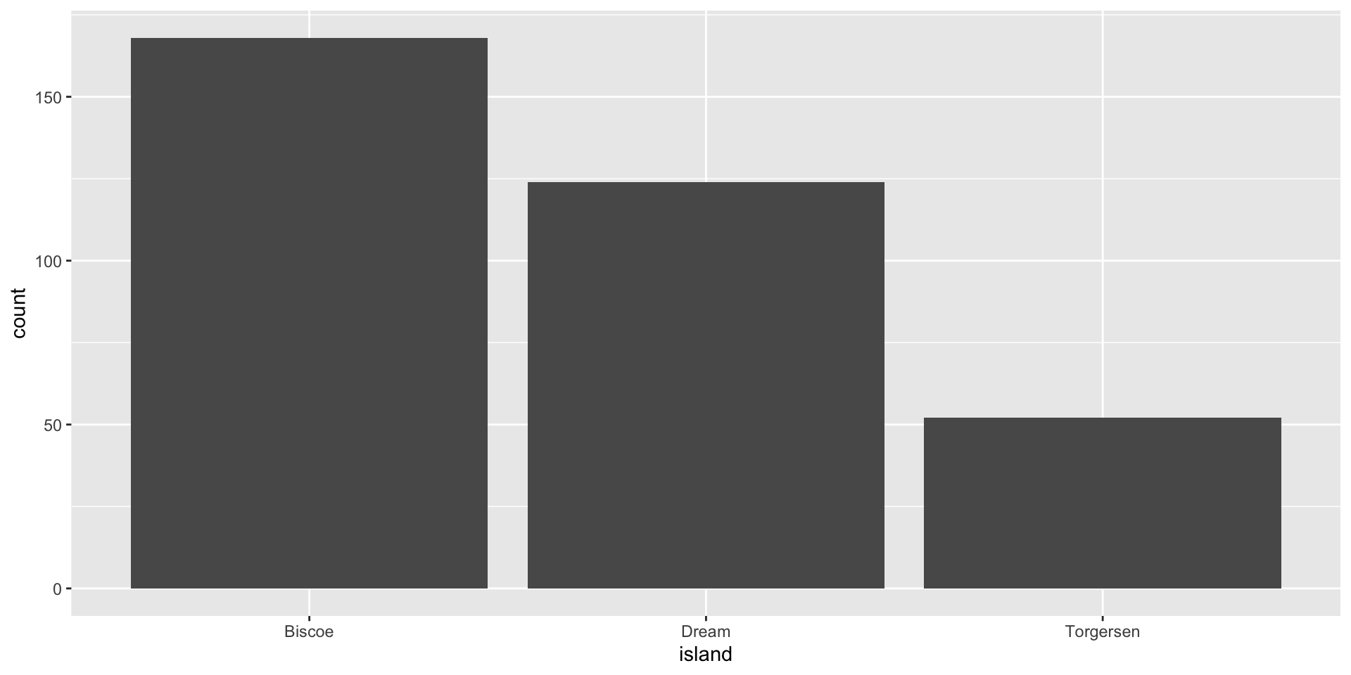
• If you have a categorical variable, then you usually want to study the frequency of its categories.
• Here the stat = "count" is computing the frequencies for each category for you.

A barplot with geom_bar() with a discrete numerical variable

penguins %>% 
  # for demonstration, change 2009 to 2012
  mutate(year = ifelse(year==2009, 2012, year)) %>% 
  ggplot(aes(x = year)) +
  geom_bar()

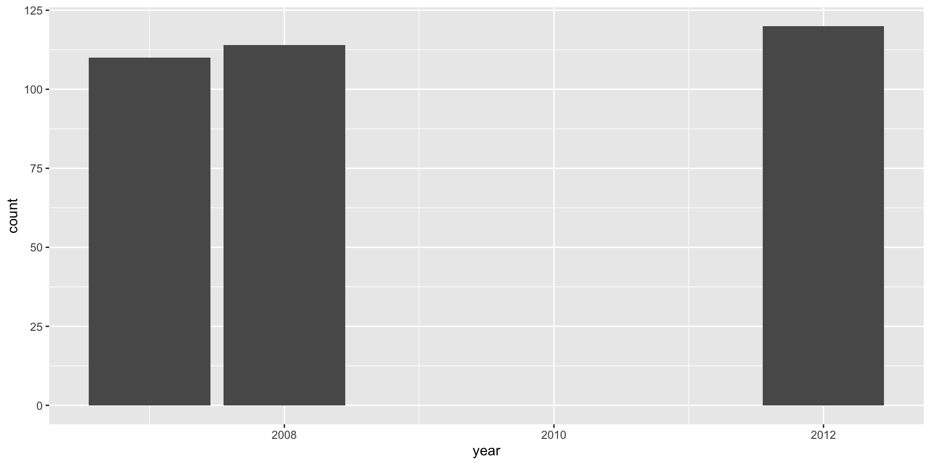
• If you supply a numerical variable, you can see now that the x-axis scale is continuous.
• If you want to study each level in a discrete variable, then you may want to convert the discrete variable to a factor instead x = factor(year).
• When the variable is a factor or character, the distances between the bars are equal and the labels correspond to that particular level.

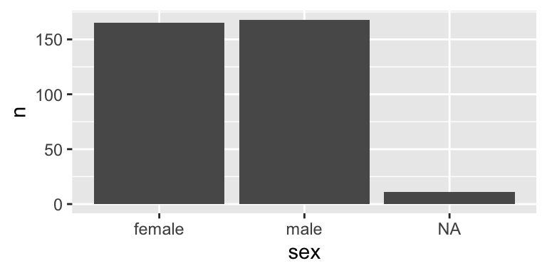
A barplot with geom_col()

• Sometimes your input data may already contain pre-computed counts.

penguins_summary <- penguins %>% group_by(sex) %>% tally() 

penguins_summary

# A tibble: 3 × 2
  sex        n
  <fct>  <int>
1 female   165
2 male     168
3 <NA>      11

• In this case, you don’t need stat = "count" to do the counting for you and use geom_col() instead.

ggplot(penguins_summary, 
       aes(x = sex, y = n)) +
  geom_col()

• This is essential a short hand for geom_bar(stat = "identity") where stat = "identity" means that you will take the value as supplied without any statistical transformation.

A stacked barplot with geom_col()

penguins %>% 
  group_by(species, sex, year) %>% 
  tally() %>% 
  ggplot(aes(year, n, fill = sex, group = year, color = species)) +
  geom_col(position = "stack", linewidth = 8) +
  geom_col(position = "stack", linewidth = 1, color = "black")

• By default the values in y are stacked on top of another.
• The aesthetic group here breaks the count in two groups and stack one on top of the other (try running the code without group = year).

A grouped barplot with geom_col()

penguins %>% 
  group_by(sex, species, year) %>% 
  tally() %>% 
  ggplot(aes(sex, n, fill = species)) +
  geom_col(color = "black", position = "dodge")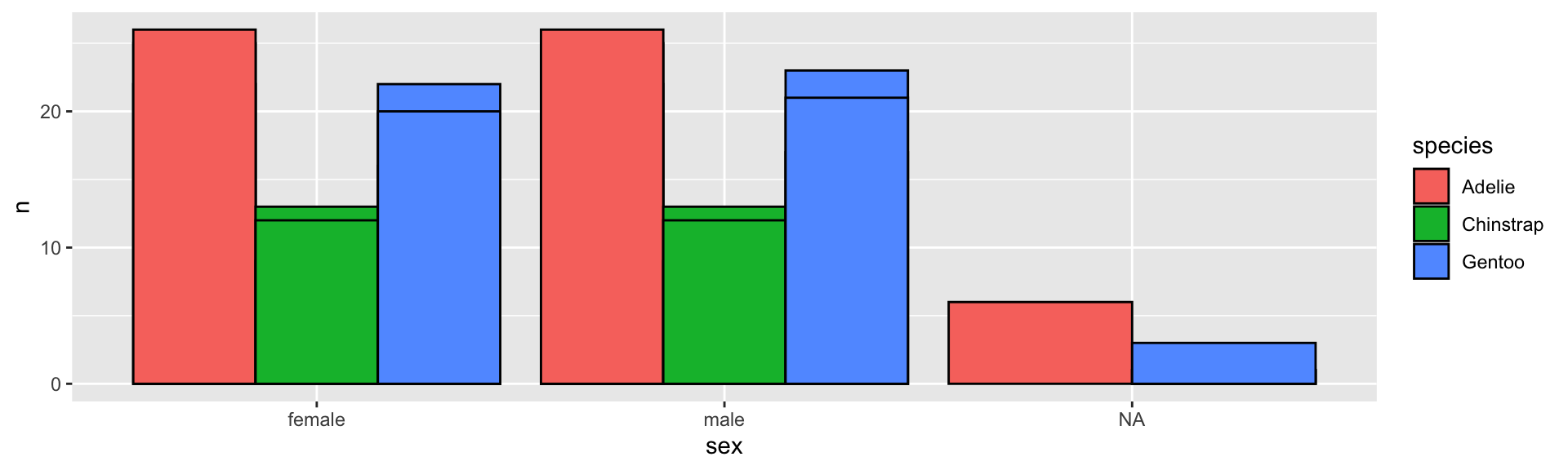

• Here the x values are recalculated so that the factor levels within the same group (as determined by x) can fit.

Another grouped barplot with geom_col()

penguins %>% 
  group_by(sex, species, year) %>% 
  tally() %>% 
  ggplot(aes(sex, n, fill = species, group = year)) +
  geom_col(color = "black", position = "dodge2")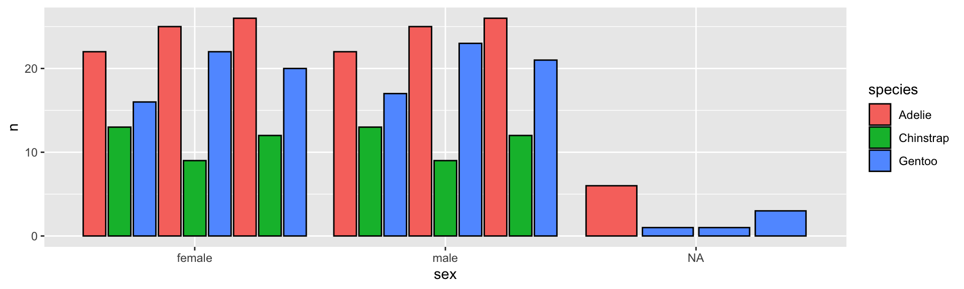

• position = "dodge" doesn’t deal well when there is fill and group together but you can use position = "dodge2" that recalculates the x values in another way.

Stacked percentage barplot with geom_col()

penguins %>% 
  group_by(species, sex, year) %>% 
  tally() %>% 
  ggplot(aes(sex, n, fill = species, group = year)) +
  geom_col(color = "black", position = "fill")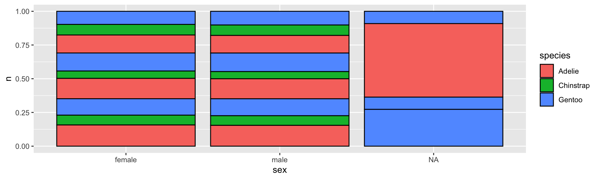

• If you want to compare the percentages between the different x, then position = "fill" can be handy.

Coordinate systems

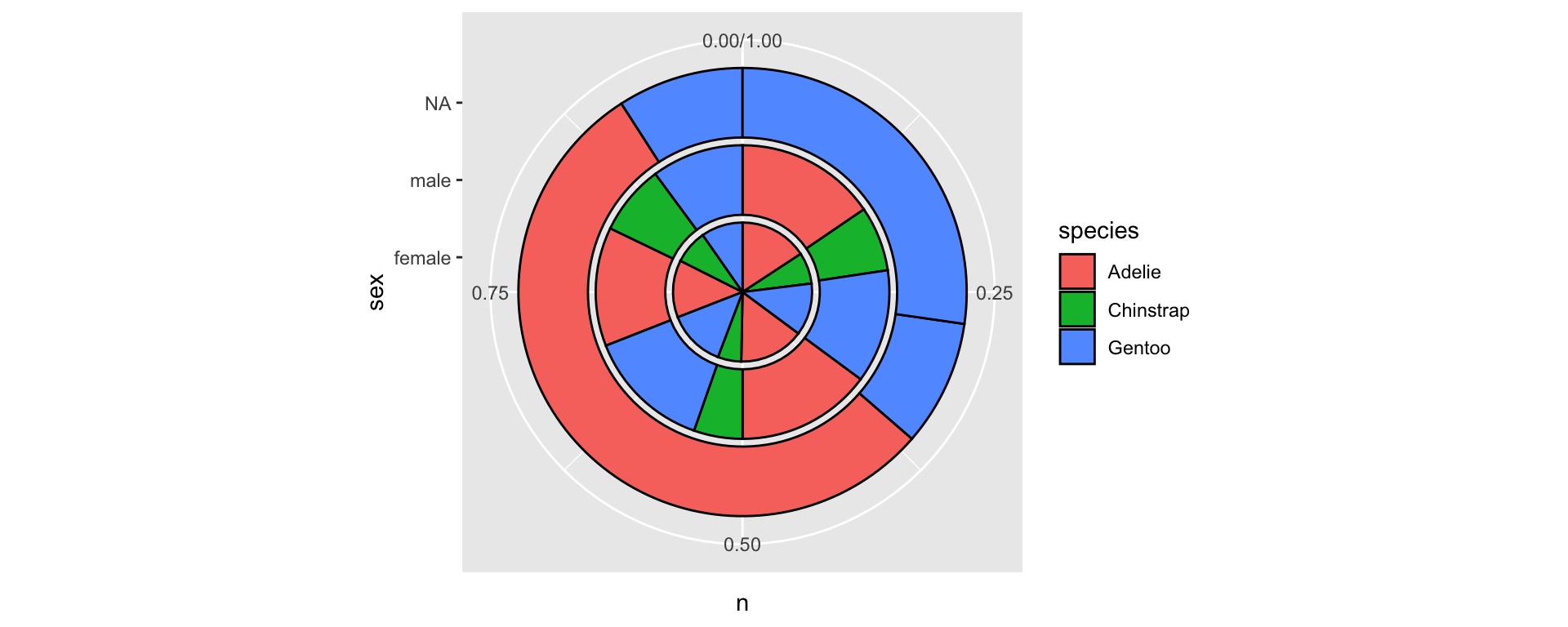
Pie or donut charts with coord_polar()

• The default coordinate system is the Cartesian coordinate system.

• But you can change this to a polar coordinate system like below.

penguins %>% 
  group_by(species, sex, year) %>% 
  tally() %>% 
  ggplot(aes(sex, n, fill = species, group = year)) +
  geom_col(color = "black", position = "fill") +
  coord_polar("y")

Other coordinate systems

• coord_cartesian() for Cartesian coordinate systems (default)
• coord_flip() to flip the x and y
• coord_fixed() to use a fixed aspect ratio
• coord_equal() is essentially coord_fixed(ratio = 1)
• coord_trans() to transform the coordinate after the statistical transformation
• coord_map() to use projection based on mapproj

Your turn!

10:00

> Go to emitanaka.org/dataviz-workshop/exercises/
> Click Exercise 4