Simple linear regression
STAT1003 – Statistical Techniques
Dr. Emi Tanaka
Australian National University
These slides are best viewed on a modern browser like Google Chrome on a desktop or laptop. Some interactive components may require some time to fully load.
Case: Seed weight from seed length
- Seed length is expected to be a major contributor to differences in seed weight for wheat.
- 190 seeds selected at random from a line of diploid wheat, Triticum monococcum for length and weight.
We seek to model the relationship between:
- the mean of a response variable, \(y\), and
- a single explanatory variable (or predictor/covariate) \(x\) as:
\[y = f(x) = \beta_0 + \beta_1 x.\]
Simple linear regression
- Suppose we have a bivariate data set \(\{(x_i, y_i)\}_{i=1}^n\) where \(x_i\) is the value of the explanatory variable and \(y_i\) is the value of the response variable for the \(i\)-th observation.
- For observations \(i = 1, 2, \ldots, n\):
\(y_i =\) \(\beta_0\) \(+\) \(\beta_1\)\(x_i +\) \(\epsilon_i\)
- \(\boldsymbol{\beta} = \begin{bmatrix}\beta_0 \\ \beta_1\end{bmatrix}\) are referred to as the regression parameters/coefficients.
- We often assume \(\epsilon_i \stackrel{iid}{\sim} N(0, \sigma^2)\), i.e. independent and identically distributed as Normal distribution of mean 0 and variance \(\sigma^2\).
intercept slope error for the \(i\)-th observation
Residual sum of squares
- Find \(\hat \beta_0\) and \(\hat \beta_1\) that minimize the sum of squares:
\[\text{RSS}(\beta_0, \beta_1) = \sum_{i=1}^n \left(\underbrace{y_i - (\beta_0 + \beta_1 x_i)}_{\text{residual}}\right)^2\]
- The least squares estimates can be found by using calculus.
- Visually, we can try changing the regression parameters below:
Least squares estimates
\[\begin{align*} \frac{\partial \text{RSS}}{\partial \beta_0} &= -2\sum_{i=1}^n \left(y_i - (\beta_0 + \beta_1 x_i)\right) = 0\\ \frac{\partial \text{RSS}}{\partial \beta_1} &= -2\sum_{i=1}^n x_i \left(y_i - (\beta_0 + \beta_1 x_i)\right) = 0 \end{align*}\]
Solving the above equations gives the least squares estimates:
\[\begin{align*} \hat{\beta}_1 &= \frac{\sum_{i=1}^n (x_i - \bar{x})(y_i - \bar{y})}{\sum_{i=1}^n (x_i - \bar{x})^2} = \frac{s_{xy}}{s_x^2}\\ \hat{\beta}_0 &= \bar{y} - \hat{\beta}_1 \bar{x} \end{align*}\]
where:
- \(s_{xy} = \frac{1}{n - 1}\sum_{i=1}^n (x_i - \bar{x})(y_i - \bar{y})\) is the sample covariance between \(x\) and \(y\), and
- \(s_x^2 = \frac{1}{n - 1}\sum_{i=1}^n (x_i - \bar{x})^2\) is the sample variance of \(x\).
- \(\bar{x} = \frac{1}{n}\sum_{i=1}^n x_i\) and \(\bar{y} = \frac{1}{n}\sum_{i=1}^n y_i\) are the sample means of \(x\) and \(y\), respectively.
Fitting linear models with R
\[\texttt{Weight}_i=\beta_0 + \beta_1\texttt{Length}_i + e_i\]
- Recall: \(\hat{\beta}_1 = \frac{s_{xy}}{s_x^2}\) and \(\hat{\beta}_0 = \bar{y} - \hat{\beta}_1 \bar{x}\).
- The least square estimates are: \(\hat{\beta}_0 = -27.93\) and \(\hat{\beta}_1 = 17.17\).
Model objects in R
- When you fit a model, you often get a model object.
- What does
fiteven contain?
- There are often methods to extract the information you need from the model object, such as
coef(),fitted(),predict(),residuals(), andsigma().
Extracting model parameter estimates
- This gives us \(\class{highlight mark-yellow}{\hat{\beta}_0} = \bar{y} - \hat{\beta}_1 \bar{x}\) and \(\class{highlight mark-yellow}{\hat{\beta}_1} = \frac{s_{xy}}{s_x^2}\).
- But what about \(\sigma^2\)? Recall \(e_i \sim NID(0, \sigma^2)\).
- An unbiased estimate of \(\sigma^2 = \text{RSS} / (n - p)\) where \(p = 2\) for simple linear regression, can be obtained by:
Fitted values
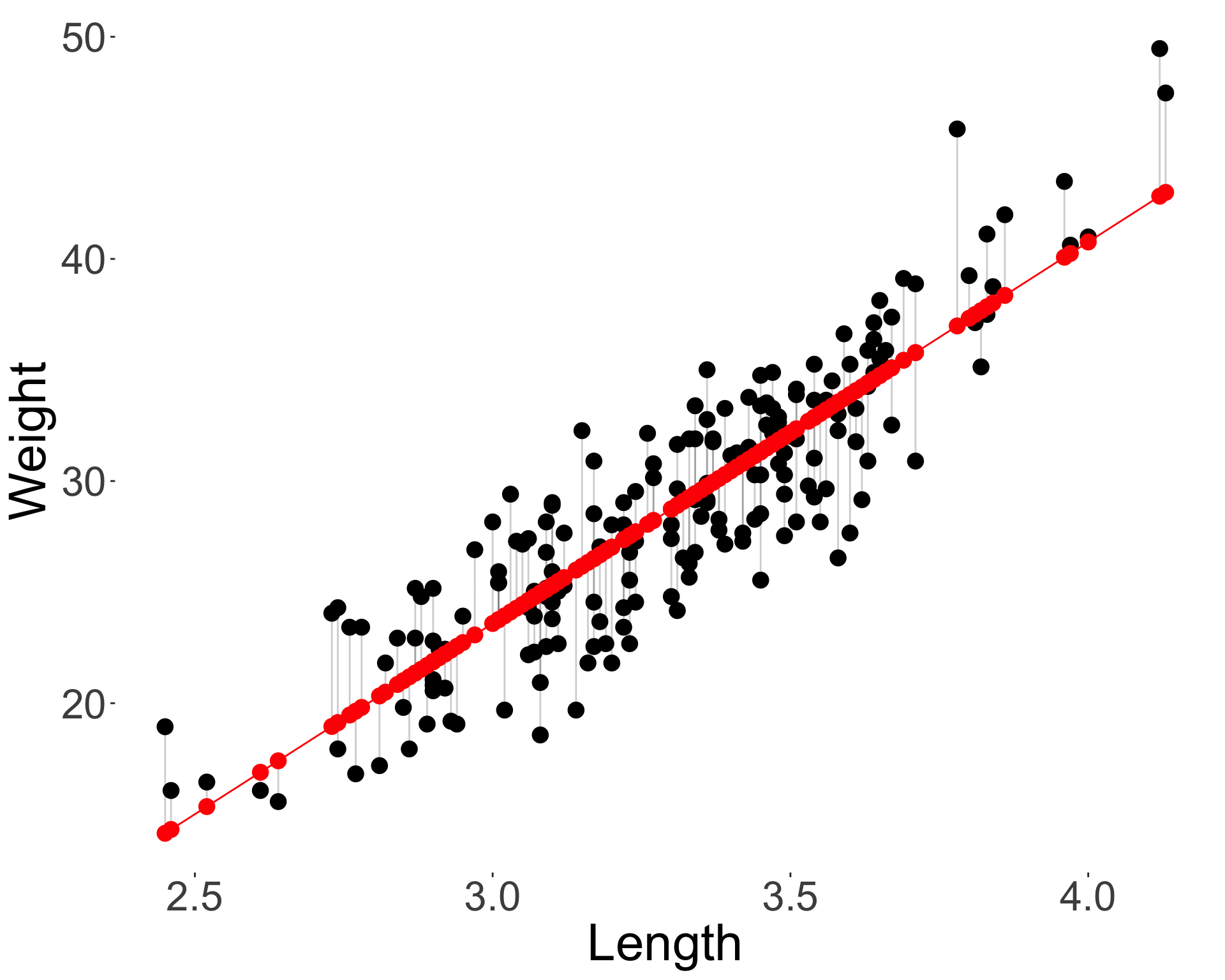
- The fitted values are the red points given as:
\[\hat{y}_i = \hat{\beta}_0 + \hat{\beta}_1 x_i.\]
Predicted values
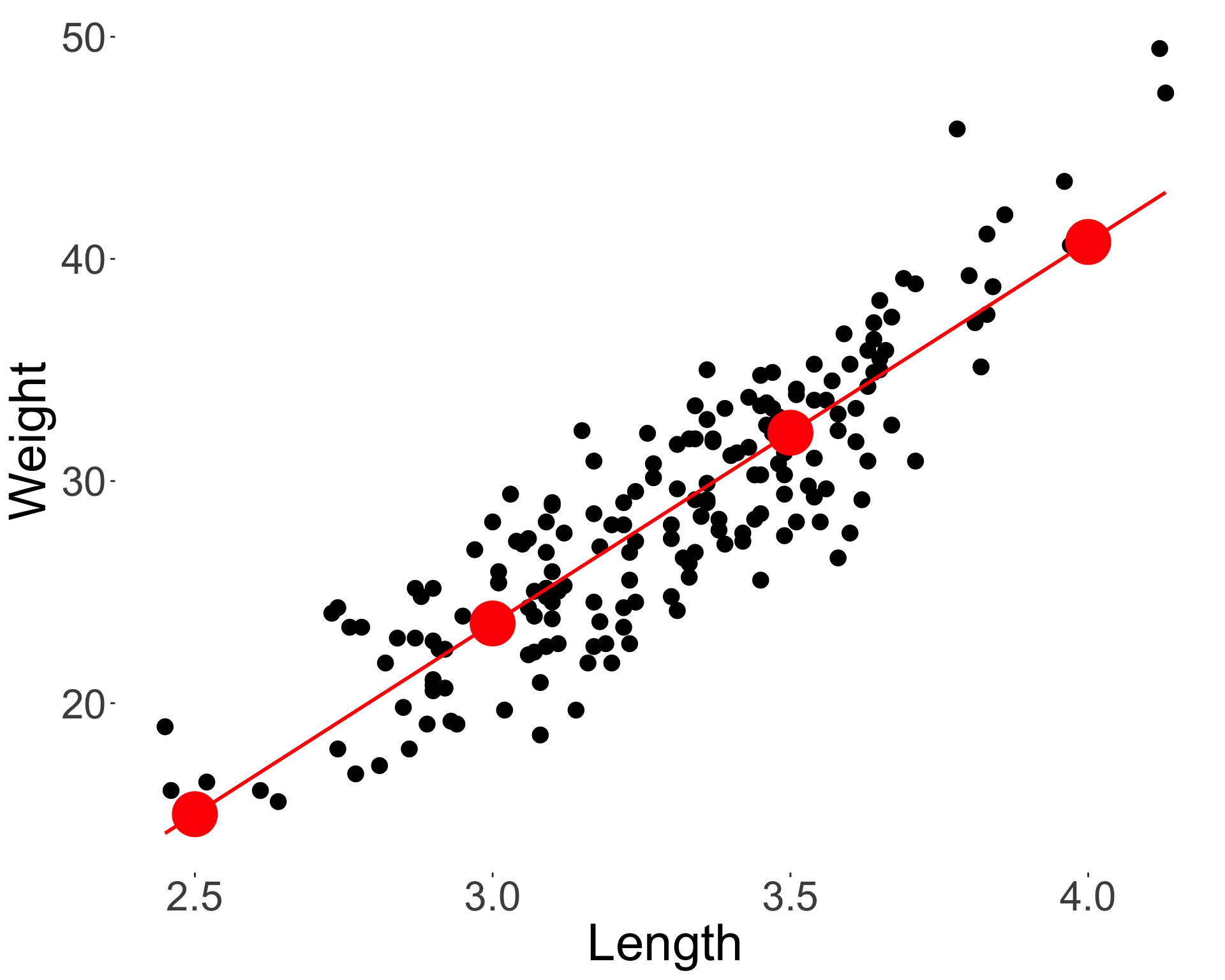
- The response can be predicted from the fitted model for a given \(x\) as:
\[\hat{y} = \hat{\beta}_0 + \hat{\beta}_1 x.\]
Residuals
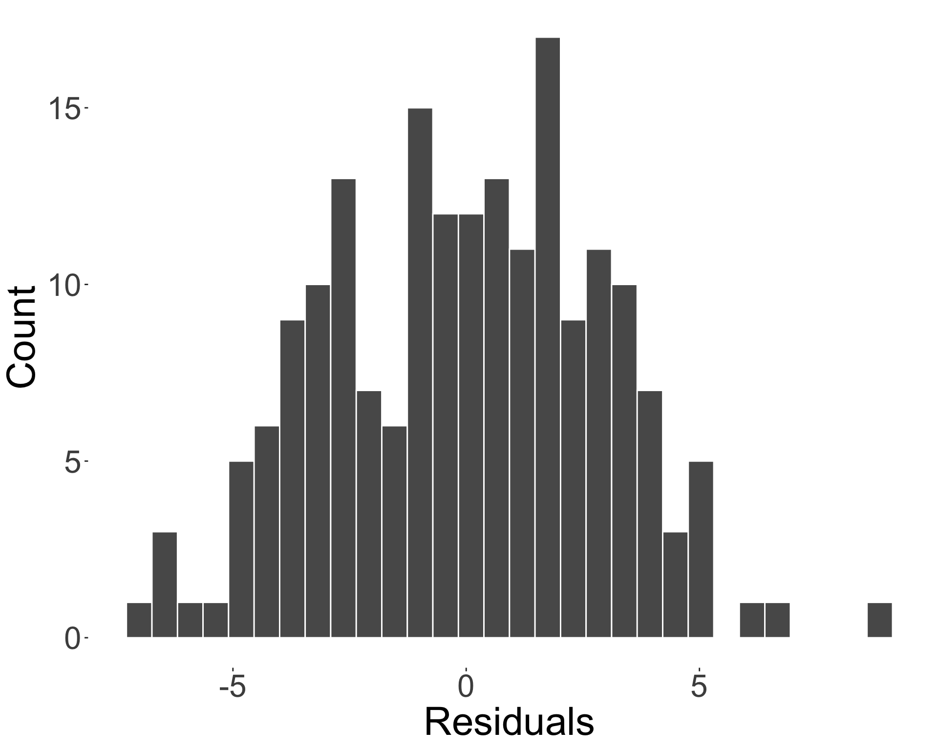
- The residuals are the vertical distances from the fitted line to the observed points, given as:
\[\hat{\epsilon}_i = y_i - \hat{y}_i = y_i - (\hat{\beta}_0 + \hat{\beta}_1 x_i).\]
Plotting linear models
geom_smooth()makes it easy to add the model to a scatter plotggpubr::stat_regline_equation()adds the regression line to the plot
Correlation coefficient and slope
Recall correlation coefficient \[r = \frac{\sum_{i=1}^n (x_i - \bar{x})(y_i - \bar{y})}{\sqrt{\sum_{i=1}^n (x_i - \bar{x})^2} \sqrt{\sum_{i=1}^n (y_i - \bar{y})^2}} = \frac{s_{xy}}{s_x s_y}\] is a measure of the strength and direction of the linear relationship between two variables.
Relationship between the slope and the correlation coefficient:
\[\hat{\beta}_1 = \frac{s_{xy}}{s_{x}^2} = \frac{s_{xy}}{s_x s_y}\frac{s_y}{s_x} = r \frac{s_y}{s_x}.\]
- Since \(s_y \geq 0\) and \(s_x \geq 0\) (but \(s_x \neq 0\) here), the sign of \(\hat{\beta}_1\) is the same as the sign of \(r\).
viewof nsample = Inputs.number([20, 1000], {step: 20, value: 200, label: "n"})
viewof intercept = Inputs.range([-10, 10], {step: 0.05, value: 0.8, label: "β₀"})
viewof slope = Inputs.range([-10,10], {step: 0.05, value: 0.8, label: "β₁"})
viewof sigma = Inputs.range([0.1, 20], {step: 0.1, value: 3, label: "σ"})
Summary
\[y_i = \beta_0 + \beta_1 x_i + \epsilon_i\]
where \(\epsilon_i \stackrel{iid}{\sim} N(0, \sigma^2)\) for \(i = 1, 2, \ldots, n\).
- \(\hat{\beta}_1 = \frac{\sum_{i=1}^n (x_i - \bar{x})(y_i - \bar{y})}{\sum_{i=1}^n (x_i - \bar{x})^2} = \dfrac{s_{xy}}{s_{x}^2} = r \dfrac{s_y}{s_x}\) and \(\hat{\beta}_0 = \bar{y} - \hat{\beta}_1 \bar{x}\).
- Fitted values: \(\hat{y}_i = \hat{\beta}_0 + \hat{\beta}_1 x_i\).
- Residuals: \(\hat{\epsilon}_i = y_i - \hat{y}_i\).
- Residual sum of squares: \(\text{RSS} = \sum_{i=1}^n \hat{\epsilon}_i^2.\)
- \(\hat{\sigma}^2 = \text{RSS} / (n - p)\) where \(p = 2\).
- The sign of \(\hat{\beta}_1\) is the same as the sign of the correlation coefficient \(r\).

STAT1003 – Statistical Techniques