Regression diagnostics

STAT1003 – Statistical Techniques

Dr. Emi Tanaka

Australian National University

These slides are best viewed on a modern browser like Google Chrome on a desktop or laptop. Some interactive components may require some time to fully load.

Table of contents

• Same regression line, different data
• Checking Assumptions
  • Assumptions for linear regression
  • (A1) \(E(\epsilon_i) = 0\)
  • (A2) Independence
  • (A3) Homoscedasticity
  • Example: Anscombe’s quartet
  • (A4) Normality
  • (A5) Predictors known without error
• Influence Measures
  • Cook’s distance
  • Leverage values for simple linear regression
  • Example: influential points in Anscombe’s quartet
• Transforming the Response
  • Box cox transformation
  • Selecting \(\lambda\) for box-cox transformation
  • Transforming the response
  • Visualizing the fitted line on the original scale
• Visual Diagnostics
  • Quick diagnostic plots
  • Visual inference
  • Visual inference for QQ-plot of residuals
• Summary

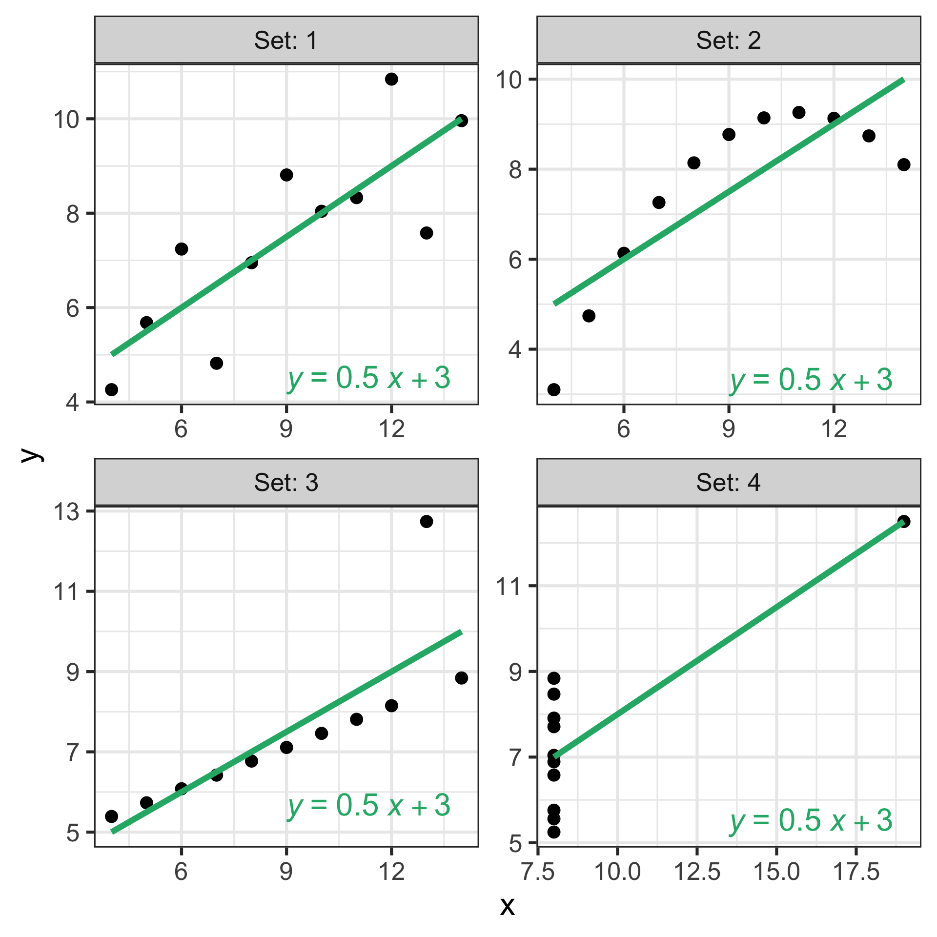
Same regression line, different data

• We can fit a regression model for any data but that doesn’t mean the model is appropriate for the data.
• All four sets of data have the same regression line (same slope and intercept) but they look very different.
• Model diagnostics is important to:
  • check the assumptions of the linear regression model are satisfied and
  • identify any potential issues with the data that may affect the validity of the model.

Anscombe, Francis J. (1973). Graphs in statistical analysis. The American Statistician, 27, 17–21.

Checking Assumptions

Assumptions for linear regression

\[y_i = \beta_0 + \beta_1 x_i + \epsilon_i, \quad i = 1, \ldots, n\]

• Recall for \(i=1,\ldots,n\), \(\epsilon_i \stackrel{iid}{\sim} N(0,\sigma^2)\) which means:
  • (A1) \(\text{E}(\epsilon_i) = 0\)
  • (A2) \(\epsilon_1, \ldots ,\epsilon_n\) are independent.
  • (A3) \(\text{Var}(\epsilon_i) = \sigma^2\) which is called the homoscedasticity assumption.
  • (A4) \(\epsilon_1, \ldots ,\epsilon_n\) are normally distributed
  • (A5) the predictors are known without error.

(A1) \(E(\epsilon_i) = 0\)

• A1 is satisfied by definition for the least squares estimates if intercept is included.

\[\sum_{i=1}^n \hat{\epsilon}_i = \sum_{i=1}^n (y_i - \underbrace{(\hat{\beta}_0 + \hat{\beta}_1 x_i)}_{\hat{y}_i}) = n\bar{y} - n\hat{\beta}_0 - n\hat{\beta}_1 \bar{x}= n\underbrace{(\bar{y}- \hat{\beta}_1 \bar{x)}}_{\hat{\beta}_0} - n\hat{\beta}_0 = 0\]

(A2) Independence

• A2 is often satisfied by design – if the data are collected in a way that ensures independence (e.g., random sampling, random assignment).
• Sometimes plotting the residuals against the order of data entry can also be useful in identifying potential violations of A2.

(A3) Homoscedasticity

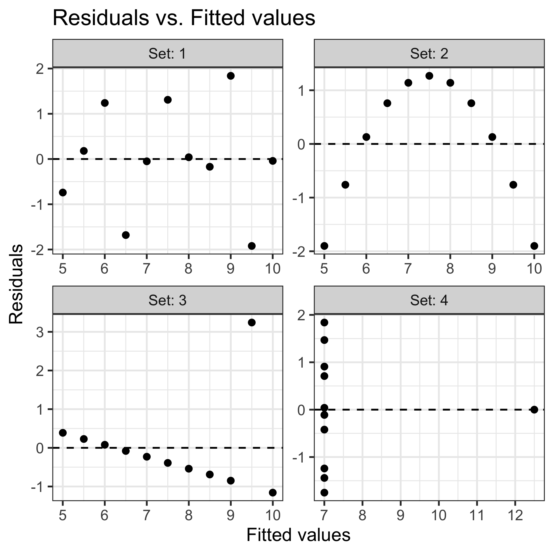
• A3 can be checked by plotting the residuals against the fitted values and ensuring that there is no pattern or trends.

• Also checked by plotting the residuals against the predictor(s) for no pattern or trends.

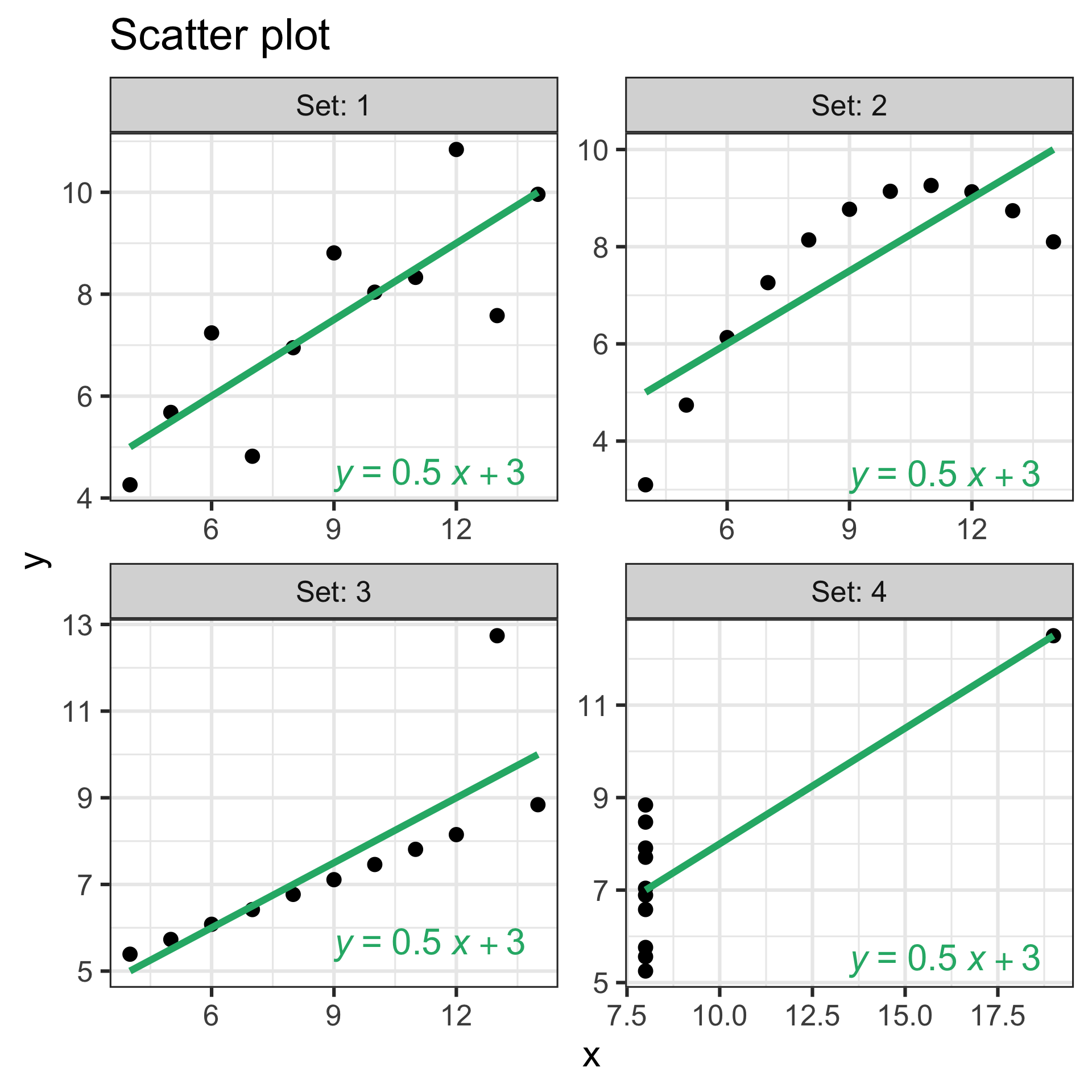
Example: Anscombe’s quartet

(A4) Normality

• If the normal quantile-quantile plot of the residuals is roughly straight then A4 is satisfied.

(A5) Predictors known without error

• There are no standard ways to check A5 easily.
• If there is measurement error in the predictor, the estimates of the regression coefficients may be biased towards zero (attenuation bias).
• If there is measurement error in the response, the estimates of the regression coefficients may be unbiased but the standard errors will be inflated, leading to less precise estimates and wider confidence intervals.

Influence Measures

Cook’s distance

The Cook’s distance for the \(i\)-th observation is defined as:

\[D_i = \frac{1}{p \hat{\sigma}^2} \sum_{j=1}^n (\hat{y}_j - \hat{y}_{j(i)})^2\]

where

• \(\hat{y}_j\) is the fitted value for the \(j\)-th observation using all data,
• \(\hat{y}_{j(i)}\) is the fitted value for the \(j\)-th observation when the \(i\)-th observation is removed from the dataset, and
• \(p\) is the number of parameters in the model (including the intercept), and
• \(\hat{\sigma}^2\) is the estimated error variance from the full model.

• \(D_i \sim F_{p, n-p}\) if the model assumptions are satisfied and the \(i\)-th observation is not influential.
• A common rule of thumb is that if \(D_i > 1\) or \(D_i > F_{0.5, p, n-p}\), then the \(i\)-th observation is considered an outlier and may warrant further investigation.

Leverage values for simple linear regression

For a simple linear regression model, the leverage values can be calculated as:

\[h_i = \frac{1}{n} + \frac{(x_i - \bar{x})^2}{\sum_{j=1}^n (x_j - \bar{x})^2}.\]

• The leverage value \(h_i\) measures how far the predictor value(s) for the \(i\)-th observation is from the mean of the predictor values.

• The leverage values range from 0 to 1.
• A common rule of thumb is that if \(h_i > 3p/n\), then the observation is considered a
  high leverage point.

Example: influential points in Anscombe’s quartet

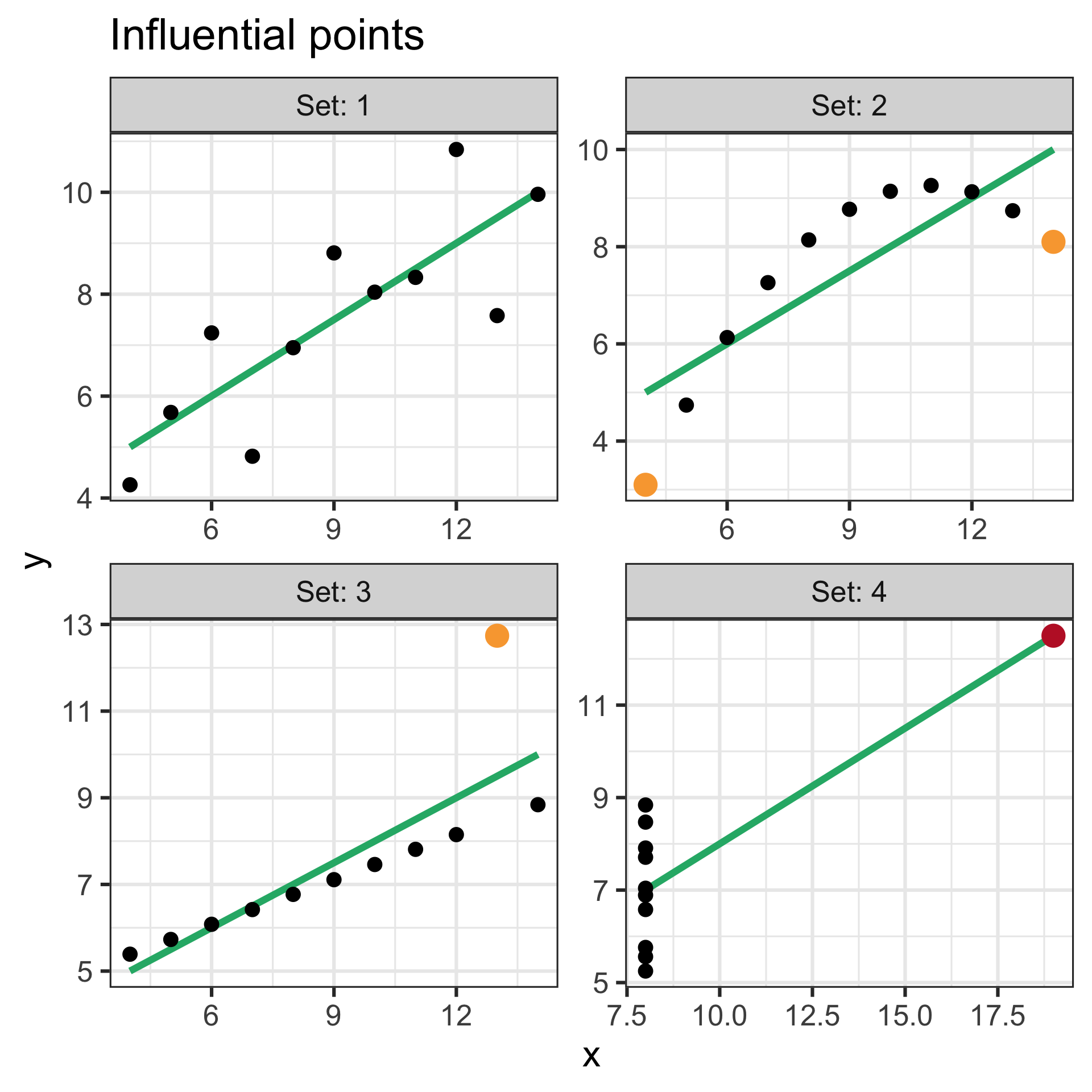
• Outliers based on Cook’s distance are highlighted in orange.
• High leverage points are highlighted in red
• These points may warrant further investigation to determine if they are data entry errors, measurement errors, or valid observations that should be retained in the analysis.
• Do not delete these points without a good reason as they may contain important information about the data and the underlying relationships between the variables.

Transforming the Response

Box cox transformation

• Box-cox transformation modifies the response for a given value of \(\lambda\) such that:

\[y(\lambda) = \begin{cases} \dfrac{y^{\lambda} - 1}{\lambda} & \text{if } \lambda \neq 0, \\ \log(y) & \text{if } \lambda = 0. \end{cases}\]

• The transformation is equivalent to:

\(\lambda\)	Transformation
\(2\)	\(y^2\)
\(1\)	\(y\)
\(0.5\)	\(\sqrt{y}\)
\(0\)	\(\log(y)\)
\(-0.5\)	\(\frac{1}{\sqrt{y}}\)
\(-1\)	\(\frac{1}{y}\)
\(-2\)	\(\frac{1}{y^2}\)

Selecting \(\lambda\) for box-cox transformation

• Profile log-likelihood plot suggests \(\lambda \approx 0.5\) which is equivalent to taking the square root of the response.

Transforming the response

• Remember the fitted or predicted value need to be squared to get the original scale.

Visualizing the fitted line on the original scale

Visual Diagnostics

Quick diagnostic plots

• An easy way to generate diagnostic plots at once is to use the ggResidpanel package.

• But the QQ-plot still doesn’t look good enough??

Visual inference

scroll

• When making inference from plots, it’s best to calibrate the plot with simulations.
• Let’s assume that \(\sqrt{\texttt{Weight}} = \hat{\beta}_0 + \hat{\beta}_1 \texttt{Length} + \epsilon\), where \(\epsilon \sim N(0, \hat{\sigma}^2)\) is the correct model.
• Then simulate from this model 17 times:

Visual inference for QQ-plot of residuals

Summary

• Model diagnostics is crucial for checking the assumptions of the linear regression model and identifying potential issues with the data.
• Common diagnostic plots include residuals vs fitted values, residuals vs predictors, and normal QQ plots of residuals.
• Influence measures such as Cook’s distance and leverage values can help identify influential observations that may warrant further investigation.
• Transforming the response variable using techniques like the Box-Cox transformation can help address violations of model assumptions.
• Visual inference using simulations can provide a more calibrated way to assess the adequacy of the visual diagnostics.