Acknowledgement

This lecture was partially adapted from the previous STAT1003 lecturers. Thank you folks!

Comparing Two Population Means

Example: rehabilitation program

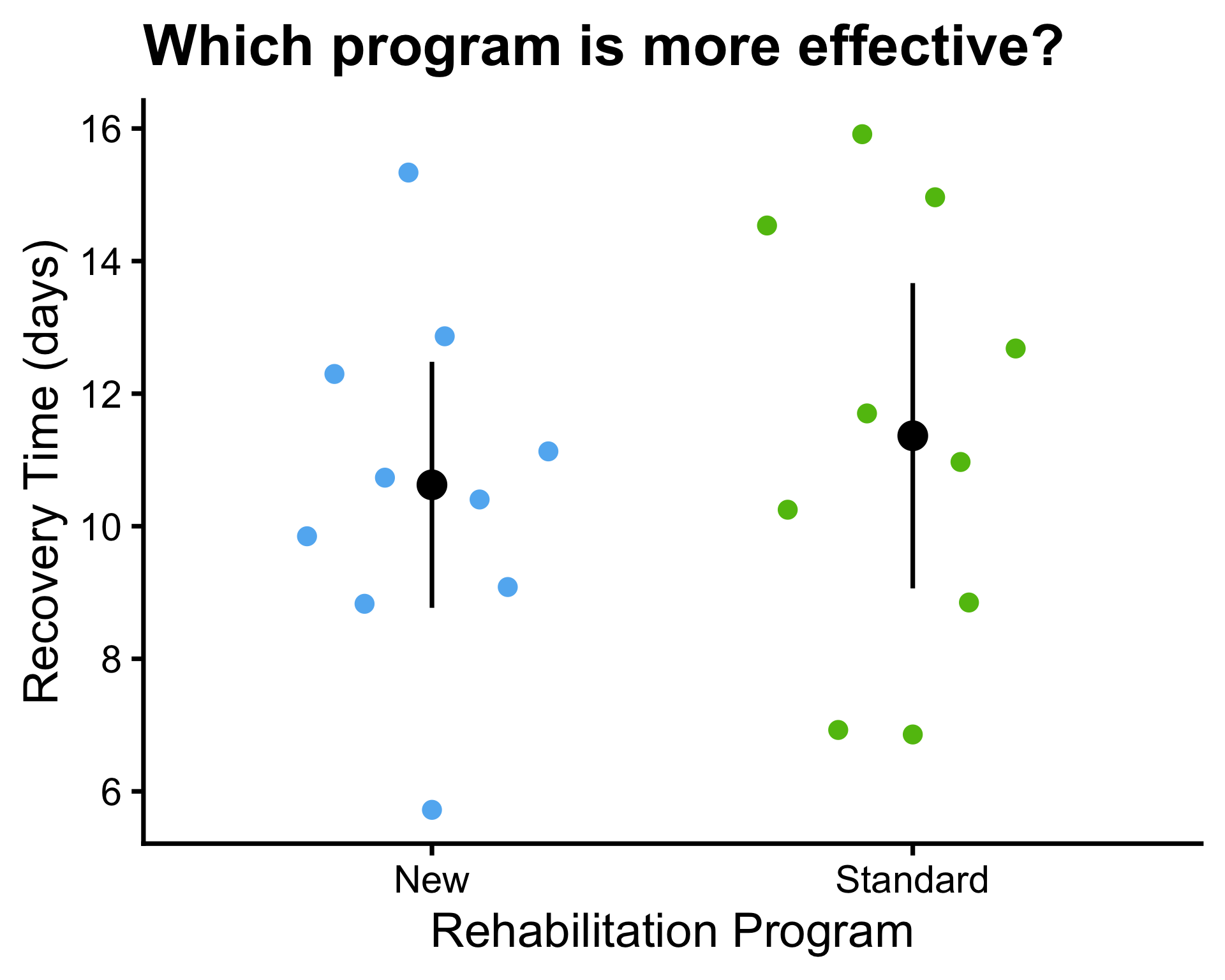
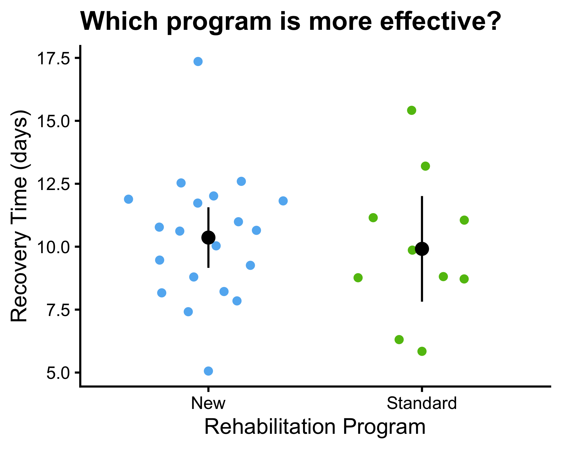
  • A hospital is comparing two rehabilitation programs (Standard and New) for patients recovering from knee surgery.
  • Patients are randomly assigned to one of the two programs.
  • The recovery time (in days) until patients can walk unassisted is recorded for each patient.

Is the new program more effective than the standard program in reducing recovery time?

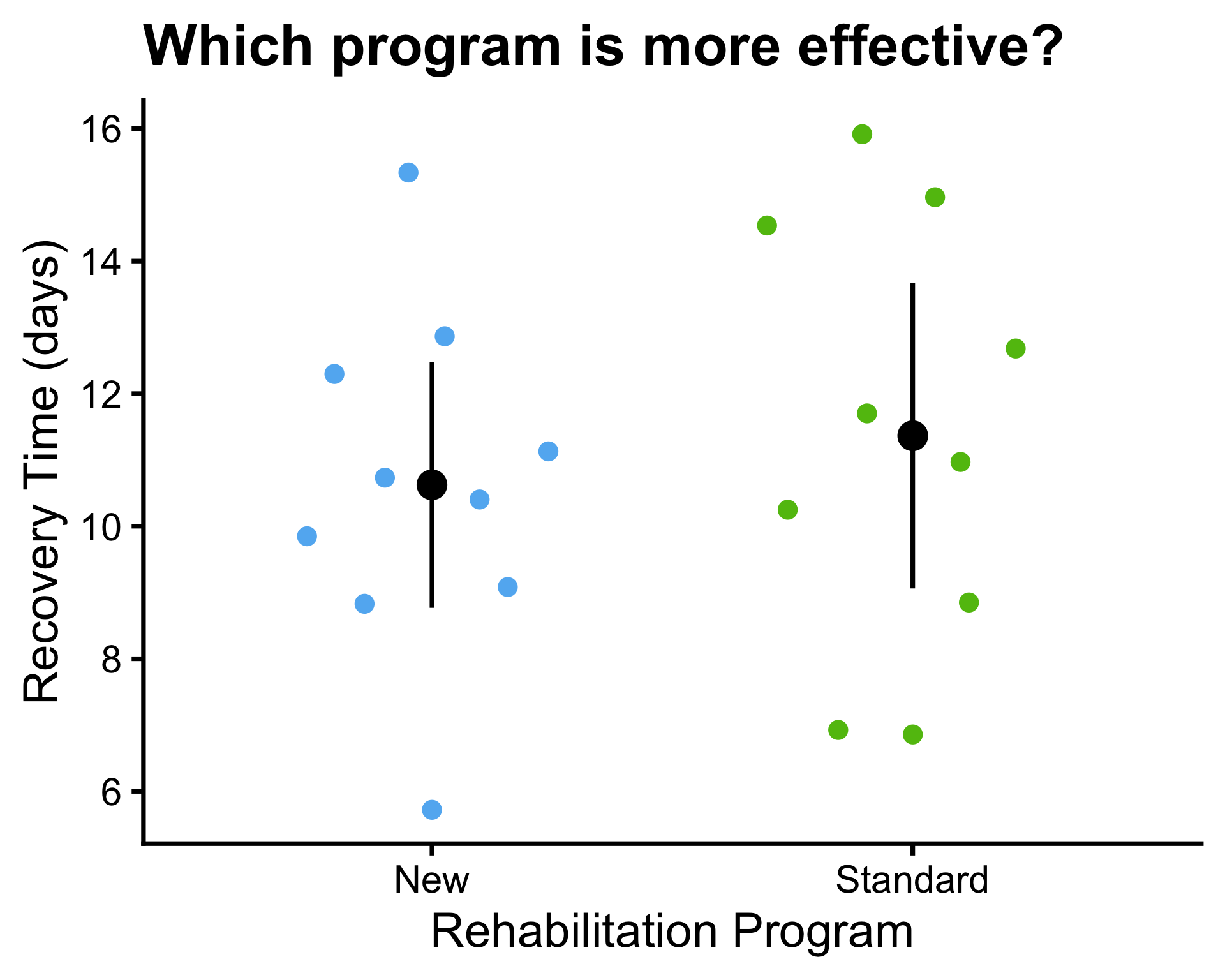
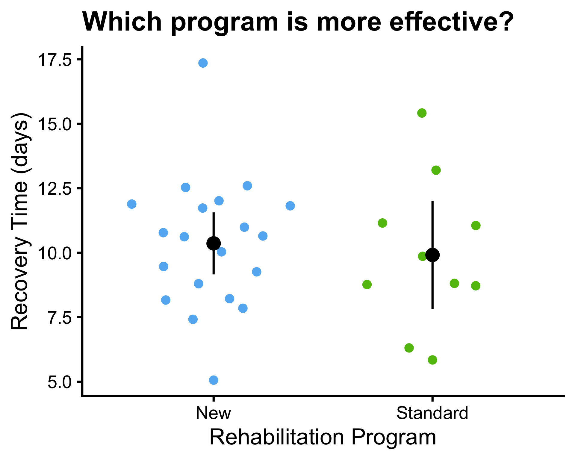
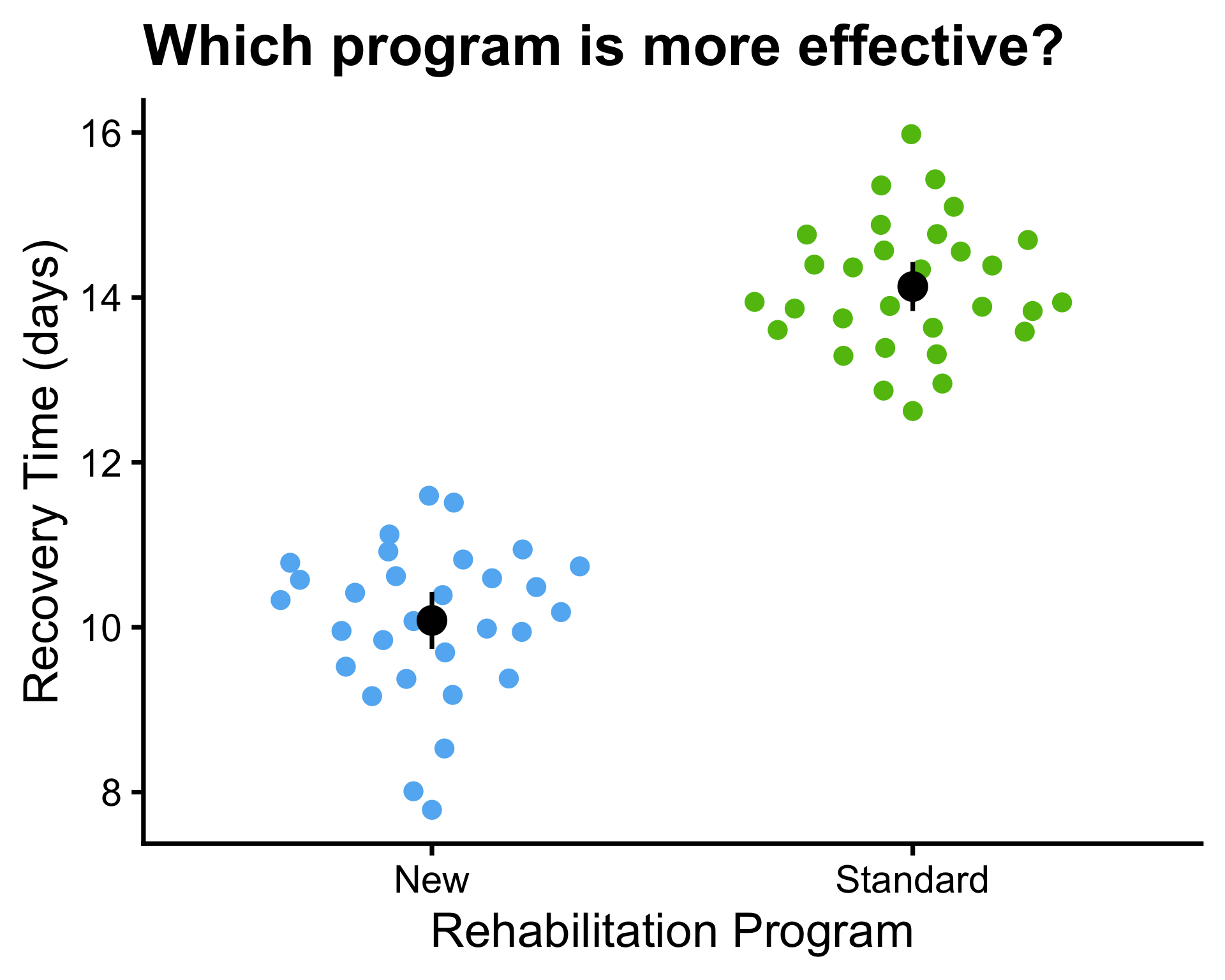
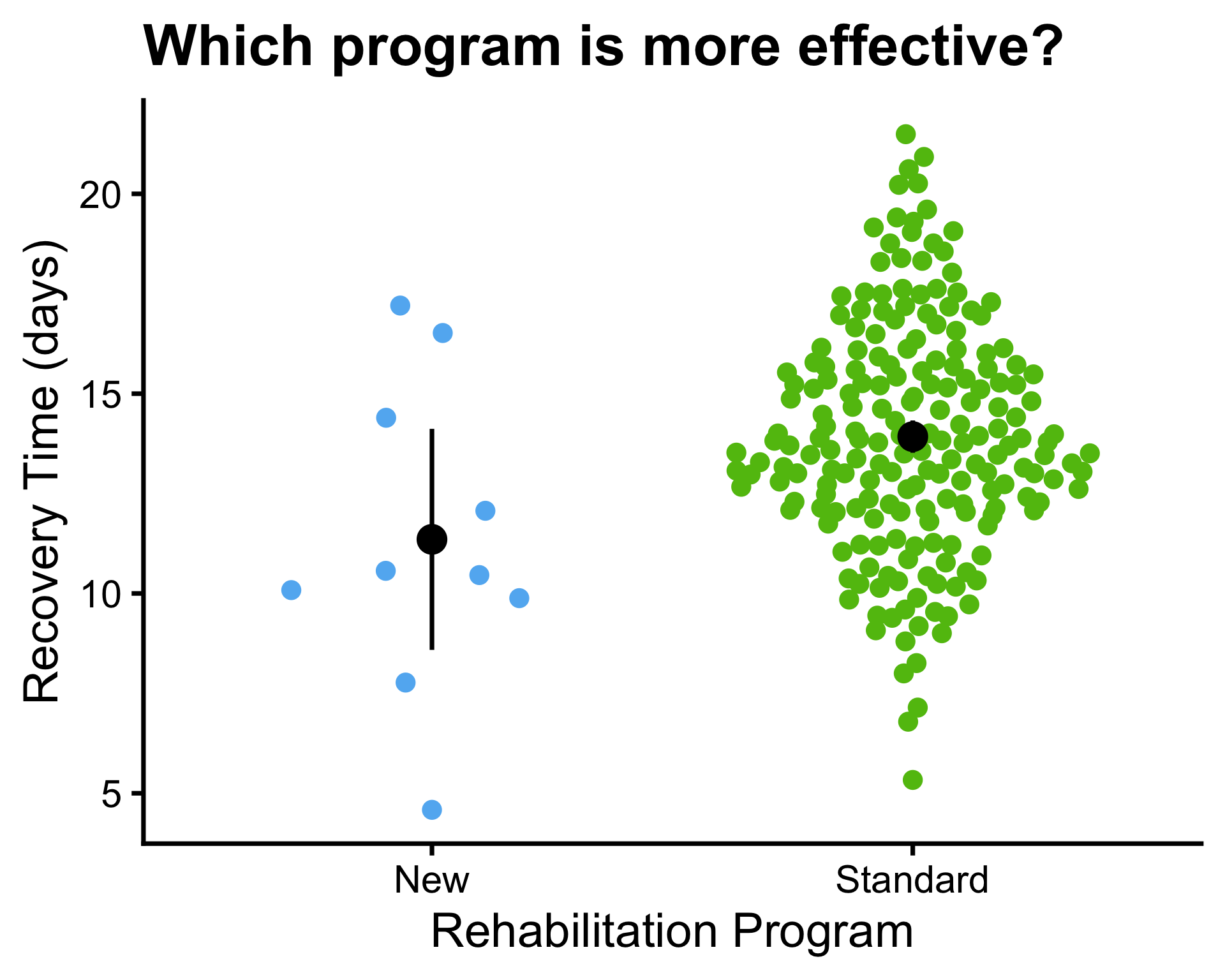
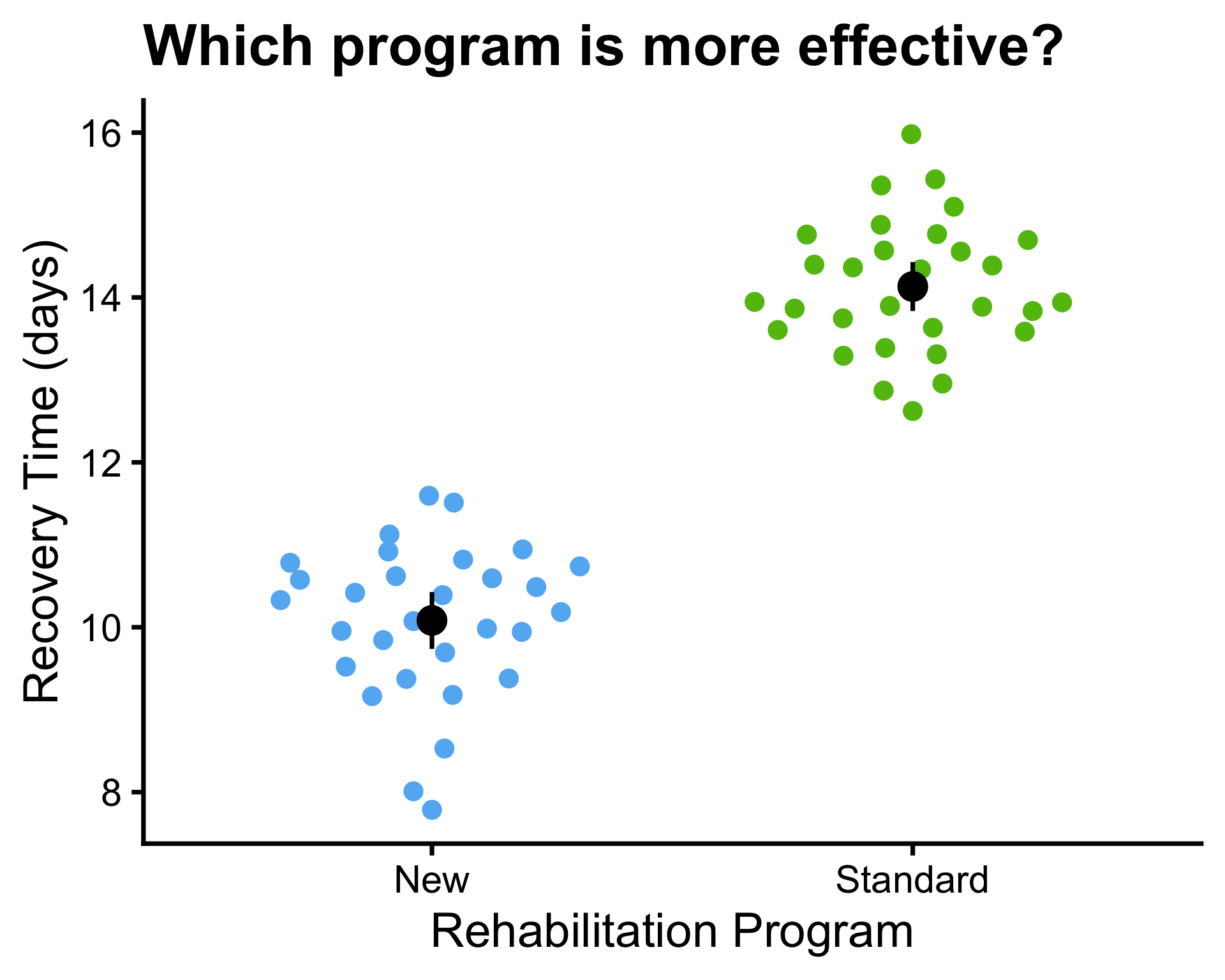
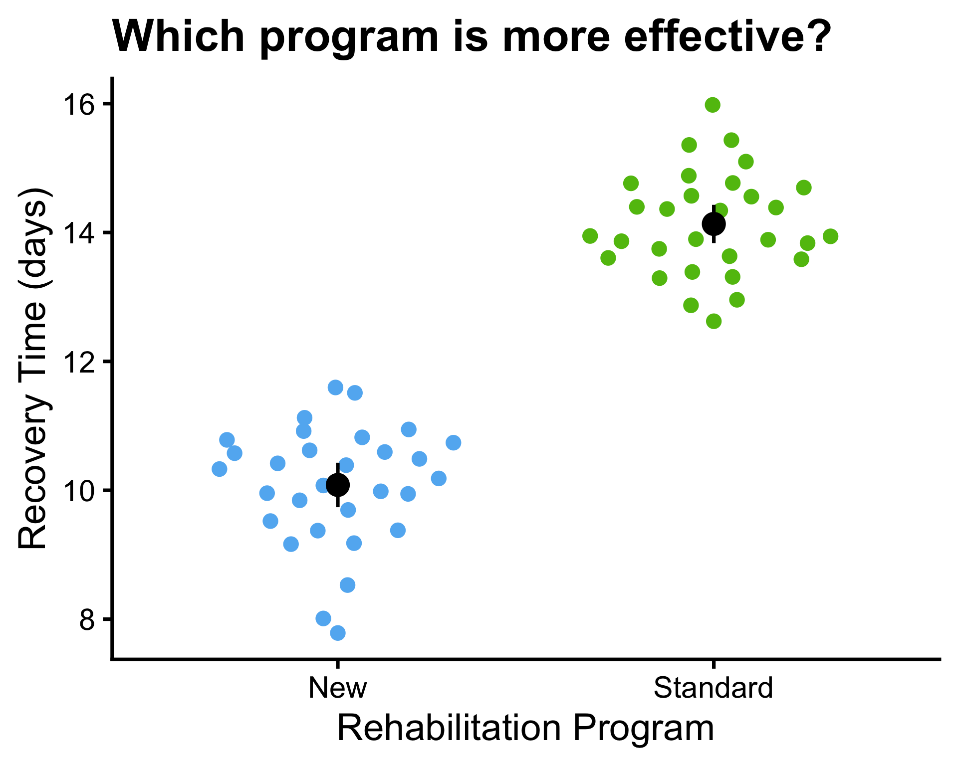
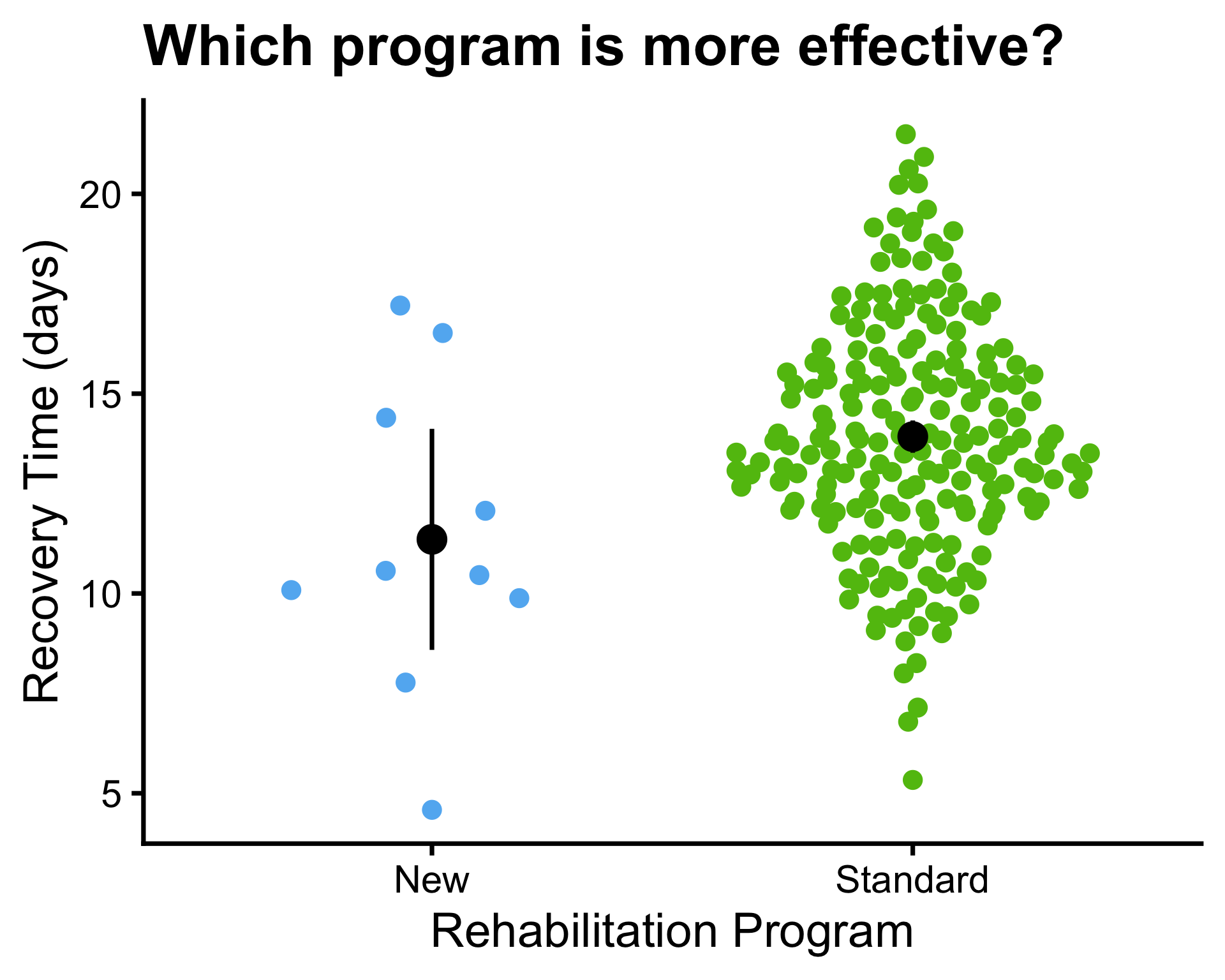
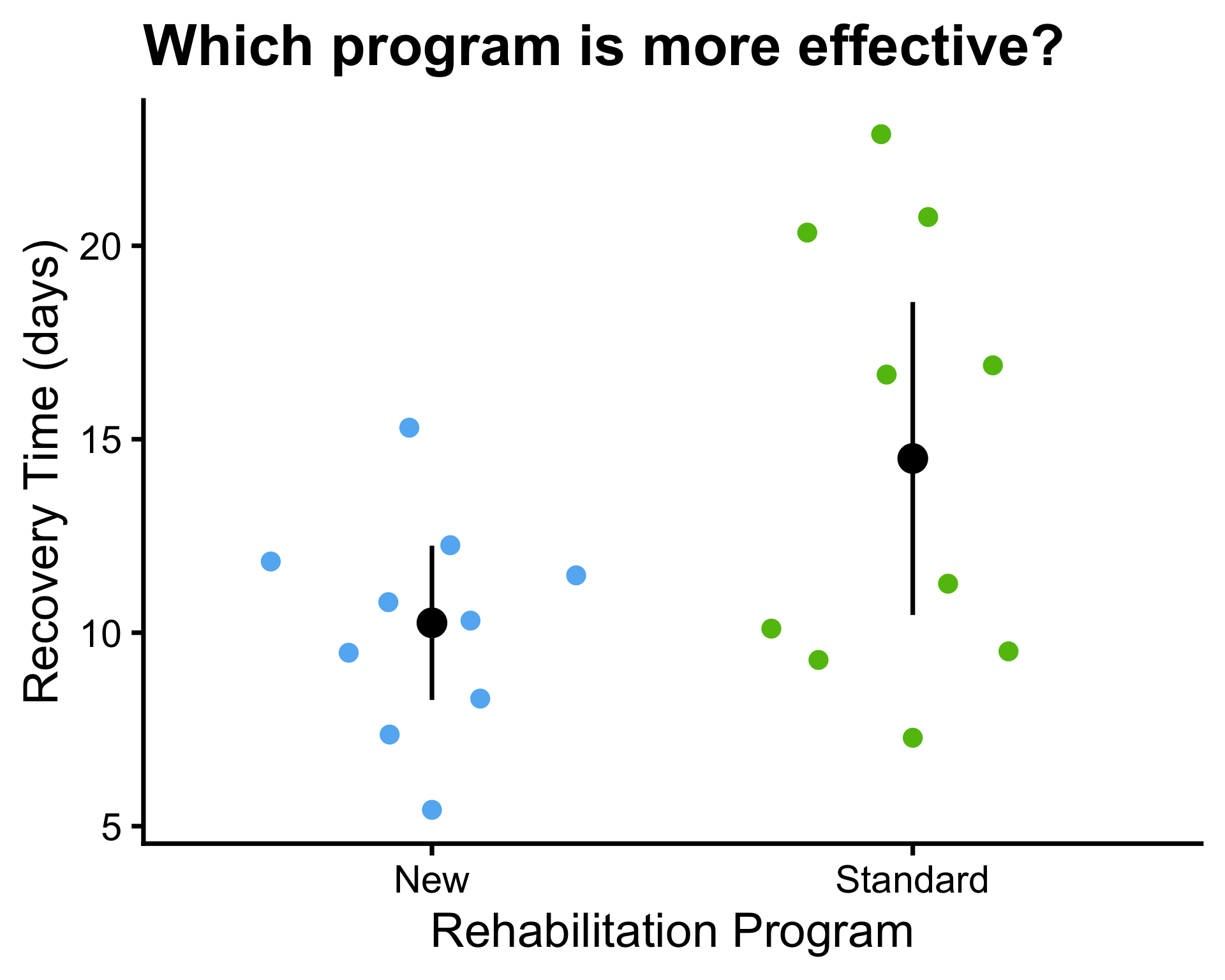
  • A beeswarm plot is a type of scatter plot that shows the distribution of a continuous variable across different groups.
  • In a beeswarm plot, the data points are arranged in a way that minimizes overlap, allowing for a clearer visualization of the distribution and density of the data within each group.
Example: hypotheses for comparing two means

Is the new program more effective than the standard program in reducing recovery time?

  • Let \(\mu_{1}\) be the mean recovery time for patients in the new rehabilitation program.
  • Let \(\mu_{2}\) be the mean recovery time for patients in the standard rehabilitation program.
  • What parameter is of interest? \(\mu_{1} - \mu_{2}\).
  • \(H_0: \mu_{1} - \mu_{2} = 0\) vs. \(H_A: \mu_{1} - \mu_{2} < 0\) (note: lower recovery time is better)
    \[\rightarrow \class{highlight mark-yellow}{H_0: \mu_{1} = \mu_{2}\quad\text{ vs. }\quad H_A: \mu_{1} < \mu_{2}}\]
  • What is a reasonable point estimator (and therefore test statistic) for \(\mu_{1} - \mu_{2}\)? \(\bar{X}_{1} - \bar{X}_{2}\).
  • What is sampling distribution of this point estimator?
  • If the samples are independent (between and within groups) and sample size is large enough (or the populations are normally distributed), then \[\class{highlight mark-yellow}{\bar{X}_{1} - \bar{X}_{2}\overset{\text{approx.}}{\sim} N\left(\mu_{1} - \mu_{2}, \frac{\sigma_1^2}{n_1} + \frac{\sigma_2^2}{n_2}\right)}\] where \(\sigma_j^2\) and \(n_j\) are the population variance and sample size for group \(j \in \{1, 2\}\), respectively.

Test statistic and its distribution

\[Z = \dfrac{(\bar{X}_{1} - \bar{X}_{2}) - (\mu_{1} - \mu_{2})}{\sqrt{\dfrac{\sigma_{1}^2}{n_{1}} + \dfrac{\sigma_{2}^2}{n_{2}}}}\]

\(Z \sim N(0, 1)\) under \(H_0: \mu_{1} = \mu_{2}\).

\[T = \dfrac{(\bar{X}_{1} - \bar{X}_{2}) - (\mu_{1} - \mu_{2})}{\sqrt{\dfrac{s_{1}^2}{n_{1}} + \dfrac{s_{2}^2}{n_{2}}}}\]

\(T \sim t_{\class{highlight mark-yellow}{\min(n_{1}, n_{2}) - 1}}\) under \(H_0: \mu_{1} = \mu_{2}\).

  • Note that the degrees of freedom above is a conservative estimate.
  • The degrees of freedom can be calculated using a more complex formula (Welch-Satterthwaite equation), but we will not cover its derivation in this course.

Special case: equal variances

  • Suppose we have reason to believe that the population variances are equal, i.e., \(\sigma_{1}^2 = \sigma_{2}^2 = \sigma^2\).
  • \(\sigma^2\) can be estimated by pooling the sample variances from the two groups: \[\class{highlight mark-yellow}{s_p^2 = \dfrac{(n_{1} - 1)s_{1}^2 + (n_{2} - 1)s_{2}^2}{n_{1} + n_{2} - 2}} = \frac{\sum_{i=1}^{n_1}(x_{i,1} - \bar{x}_{1})^2 + \sum_{i=1}^{n_2}(x_{i,2} - \bar{x}_{2})^2}{n_{1} + n_{2} - 2}\]

\[T = \dfrac{(\bar{X}_{1} - \bar{X}_{2}) - (\mu_{1} - \mu_{2})}{\sqrt{\class{highlight mark-yellow}{s_p^2}\left(\dfrac{1}{n_{1}} + \dfrac{1}{n_{2}}\right)}}\]

\(T \sim t_{\class{highlight mark-yellow}{n_{1} + n_{2} - 2}}\) under \(H_0: \mu_{1} = \mu_{2}\).

\(100(1-\alpha)\%\) confidence interval for \(\mu_{1} - \mu_{2}\)

\[\bar{X}_{1} - \bar{X}_{2} \pm z_{\alpha / 2} \sqrt{\dfrac{\sigma_{1}^2}{n_{1}} + \dfrac{\sigma_{2}^2}{n_{2}}}\]

\[\bar{X}_{1} - \bar{X}_{2} \pm t_{\text{df}, \alpha / 2} \sqrt{\dfrac{s_{1}^2}{n_{1}} + \dfrac{s_{2}^2}{n_{2}}}\]

where:

  • \(\text{df} = \min(n_{1}, n_{2}) - 1\) if variances cannot not be assumed to be equal
  • \(\text{df} = n_{1} + n_{2} - 2\) if variances are assumed to be equal and \(s^2_1 = s^2_2 = s^2_p\).

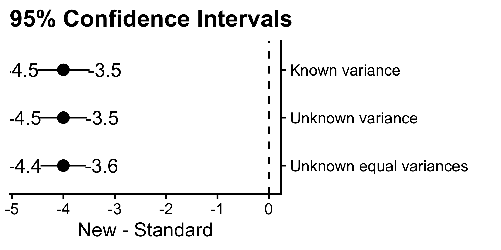
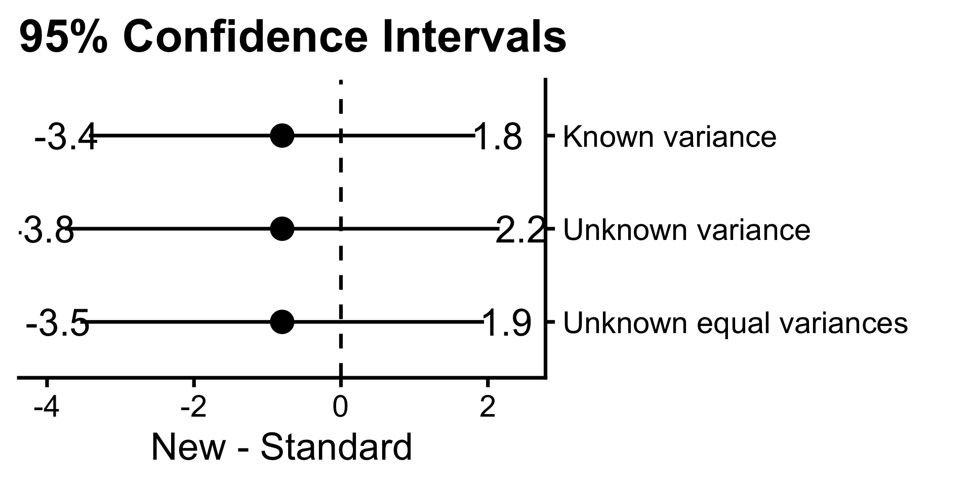
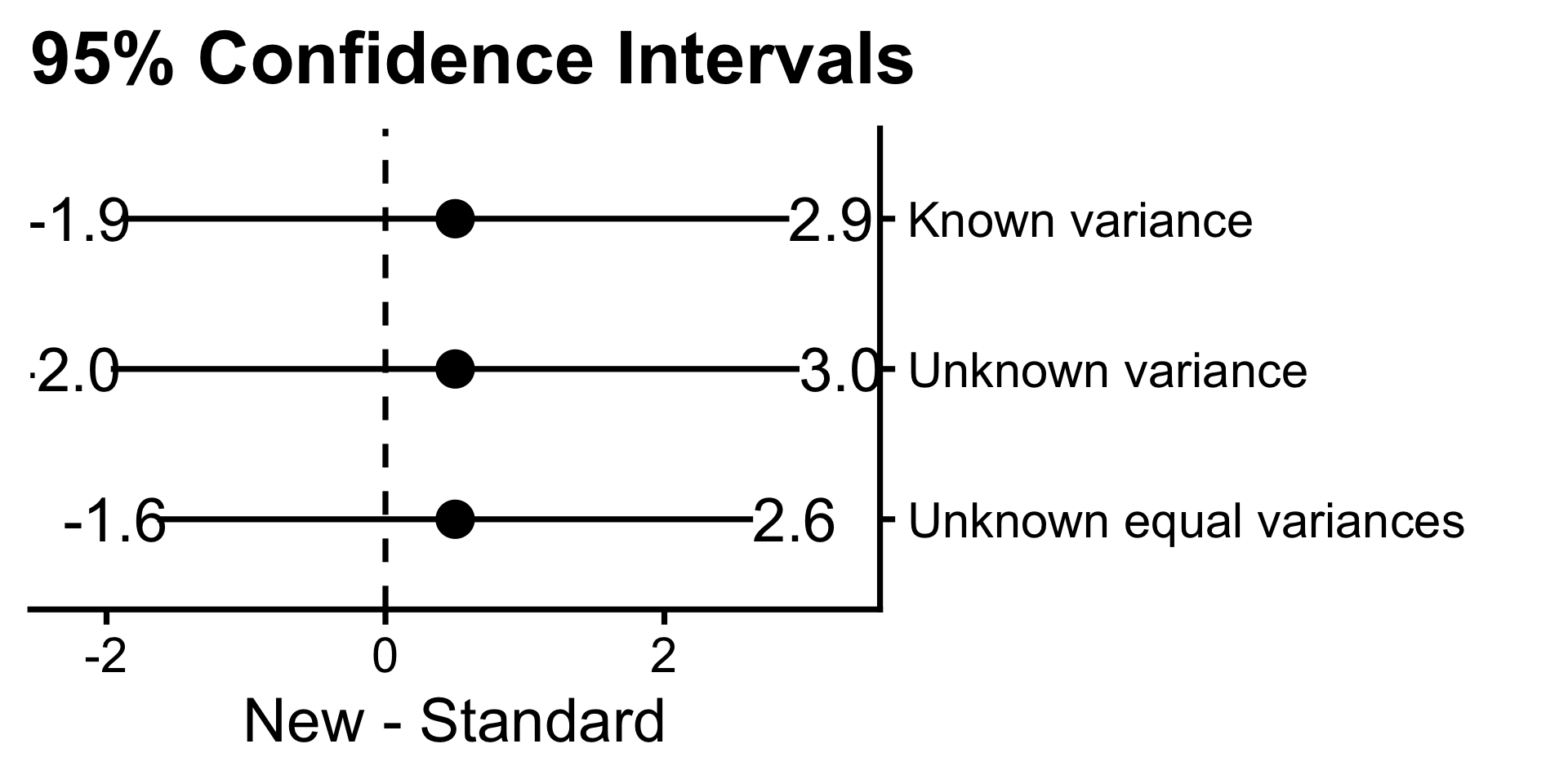
Example: 95% confidence interval

  • \(\mu_1 = 10\) and \(\mu_2 = 14\)
  • \(\bar{x}_1 = 10.1\) and \(\bar{x}_2 = 14.1\)
  • \(\sigma^2_1 = 1\) and \(\sigma^2_2 = 1\)
  • \(s_1^2 = 0.85\) and \(s_2^2 = 0.63\), \(s_p^2 = 0.74\)
  • \(n_1 = 30\) and \(n_2 = 30\)

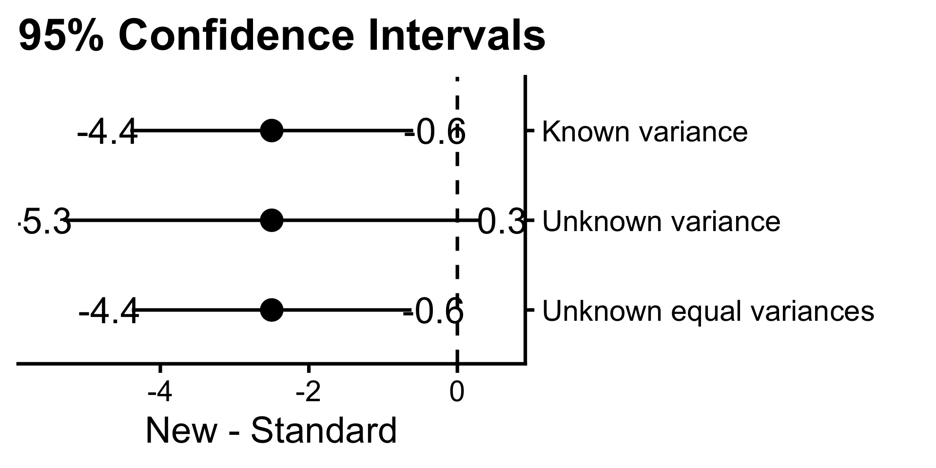
  • \(\mu_1 = 10\) and \(\mu_2 = 14\)
  • \(\bar{x}_1 = 11.4\) and \(\bar{x}_2 = 13.9\)
  • \(\sigma^2_1 = 9\) and \(\sigma^2_2 = 9\)
  • \(s_1^2 = 14.95\) and \(s_2^2 = 8.4\), \(s_p^2 = 8.69\)
  • \(n_1 = 10\) and \(n_2 = 200\)

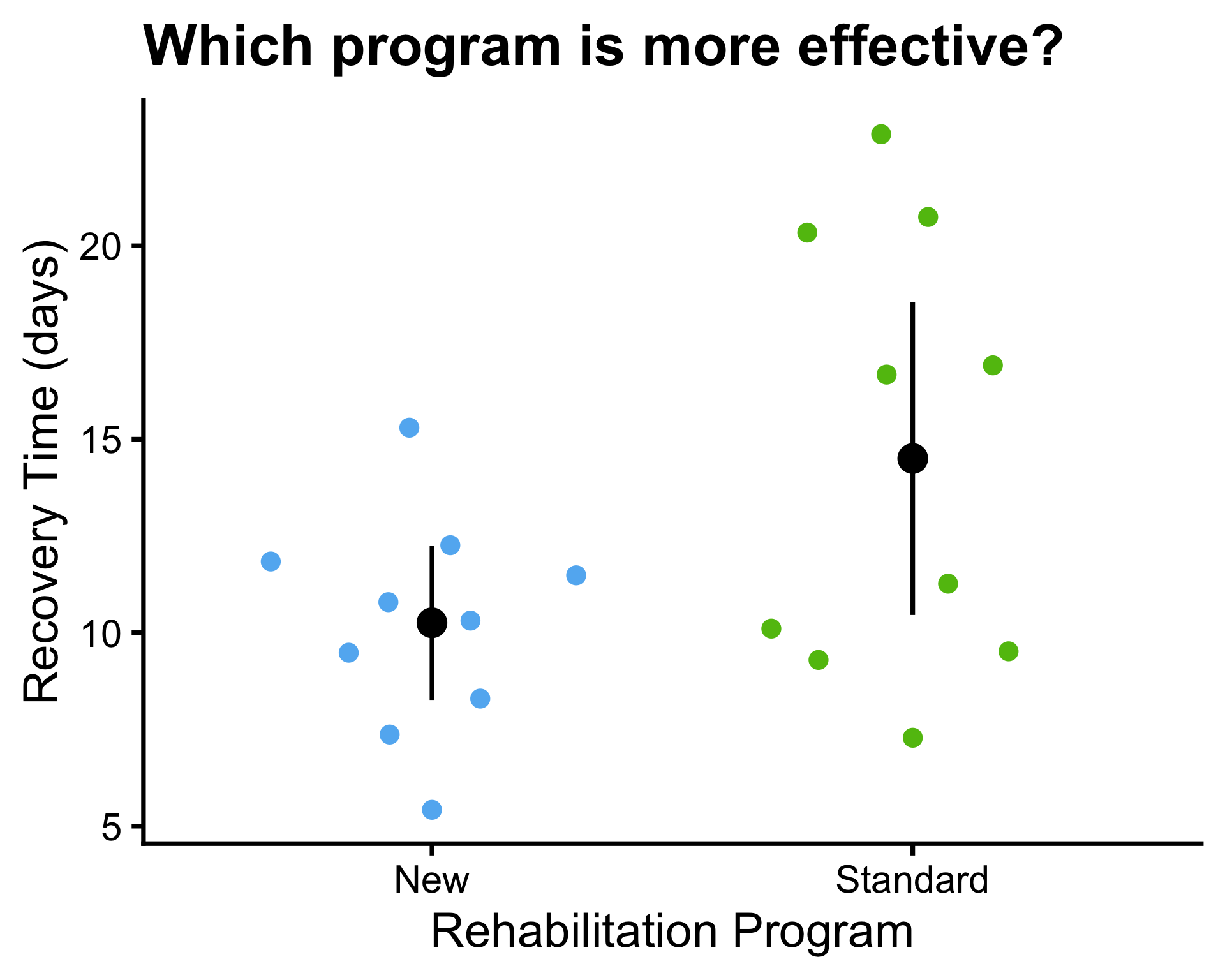
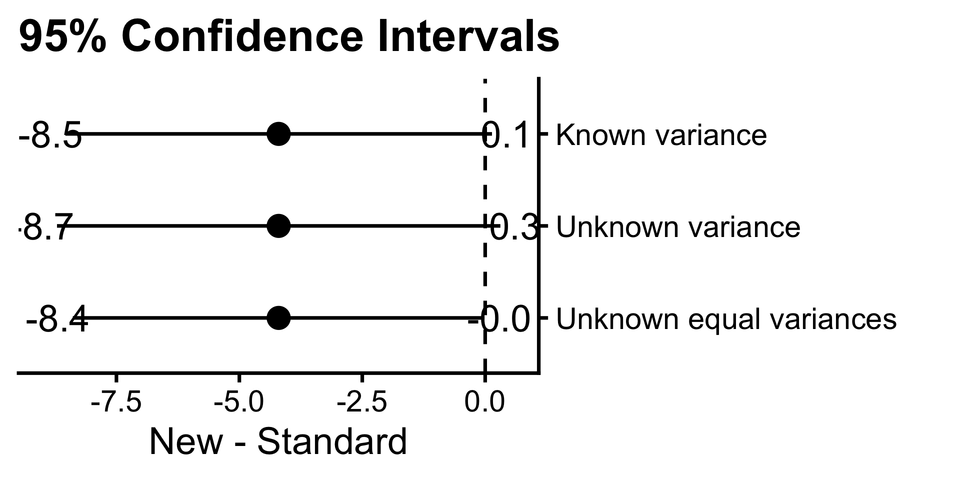
  • \(\mu_1 = 10\) and \(\mu_2 = 14\)
  • \(\bar{x}_1 = 10.3\) and \(\bar{x}_2 = 14.5\)
  • \(\sigma^2_1 = 4\) and \(\sigma^2_2 = 45\)
  • \(s_1^2 = 7.77\) and \(s_2^2 = 31.96\), \(s_p^2 = 19.86\)
  • \(n_1 = 10\) and \(n_2 = 10\)

  • \(\mu_1 = 10\) and \(\mu_2 = 10\)
  • \(\bar{x}_1 = 10.6\) and \(\bar{x}_2 = 11.4\)
  • \(\sigma^2_1 = 9\) and \(\sigma^2_2 = 9\)
  • \(s_1^2 = 6.73\) and \(s_2^2 = 10.37\), \(s_p^2 = 8.55\)
  • \(n_1 = 10\) and \(n_2 = 10\)

  • \(\mu_1 = 10\) and \(\mu_2 = 10\)
  • \(\bar{x}_1 = 10.4\) and \(\bar{x}_2 = 9.9\)
  • \(\sigma^2_1 = 9.89\) and \(\sigma^2_2 = 10\)
  • \(s_1^2 = 6.61\) and \(s_2^2 = 8.61\), \(s_p^2 = 7.25\)
  • \(n_1 = 20\) and \(n_2 = 10\)

Hypothesis testing for comparing two means

\(H_0: \mu_1 = \mu_2\)

\(z^* = \dfrac{\bar{x}_{1} - \bar{x}_{2}}{\sqrt{\dfrac{\sigma_1^2}{n_1} + \dfrac{\sigma_2^2}{n_2}}}\)

  • \(H_A: \mu_1 < \mu_2\)
    P-value \(= P(Z \leq z^*)\)
  • \(H_A: \mu_1 > \mu_2\)
    P-value \(= P(Z \geq z^*)\)
  • \(H_A: \mu_1 \neq \mu_2\)
    P-value \(= 2P(Z \geq |z^*|)\)

where \(Z \sim N(0, 1)\) under \(H_0\).

\(t^* = \dfrac{\bar{x}_{1} - \bar{x}_{2}}{\sqrt{\dfrac{s_1^2}{n_1} + \dfrac{s_2^2}{n_2}}}\)

  • \(H_A: \mu_1 < \mu_2\) \(\rightarrow\) P-value \(= P(T \leq t^*)\)
  • \(H_A: \mu_1 > \mu_2\) \(\rightarrow\) P-value \(= P(T \geq t^*)\)
  • \(H_A: \mu_1 \neq \mu_2\) \(\rightarrow\) P-value \(= 2P(T \geq |t^*|)\)

where

  • \(T \sim t_{\text{df}}\) under \(H_0\),
  • \(\text{df} = \min(n_{1}, n_{2}) - 1\) if variances cannot not be assumed to be equal, and
  • \(\text{df} = n_{1} + n_{2} - 2\) if variances are assumed to be equal and \(s^2_1 = s^2_2 = s^2_p\).

Example: p-values

  • \(\mu_1 = 10\) and \(\mu_2 = 14\)
  • \(\bar{x}_1 = 10.1\) and \(\bar{x}_2 = 14.1\)
  • \(\sigma^2_1 = 1\) and \(\sigma^2_2 = 1\)
  • \(s_1^2 = 0.85\) and \(s_2^2 = 0.63\), \(s_p^2 = 0.74\)
  • \(n_1 = 30\) and \(n_2 = 30\)

P-values:

  • Known variance: \(P(Z \leq -15.49) = 0.0000\)
  • Unknown variance: \(P(t_{29} \leq -18.01) = 0.0000\)
  • Unknown equal variances: \(P(t_{58} \leq -18.01) = 0.0000\)
  • \(\mu_1 = 10\) and \(\mu_2 = 14\)
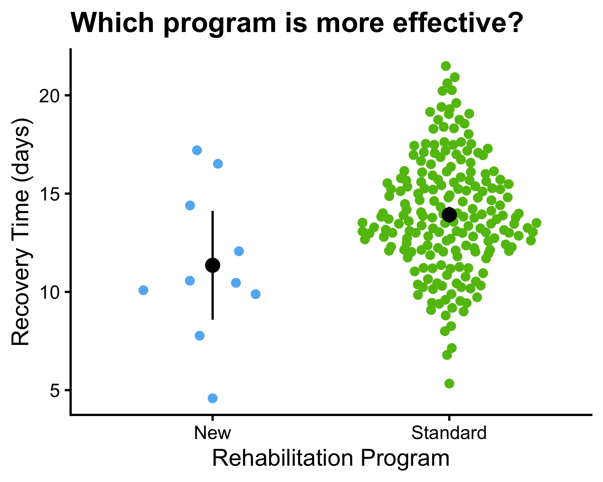
  • \(\bar{x}_1 = 11.4\) and \(\bar{x}_2 = 13.9\)
  • \(\sigma^2_1 = 9\) and \(\sigma^2_2 = 9\)
  • \(s_1^2 = 14.95\) and \(s_2^2 = 8.4\), \(s_p^2 = 8.69\)
  • \(n_1 = 10\) and \(n_2 = 200\)

P-values:

  • Known variance: \(P(Z \leq -2.57) = 0.0051\)
  • Unknown variance: \(P(t_{9} \leq -2.02) = 0.0371\)
  • Unknown equal variances: \(P(t_{208} \leq -2.62) = 0.0047\)
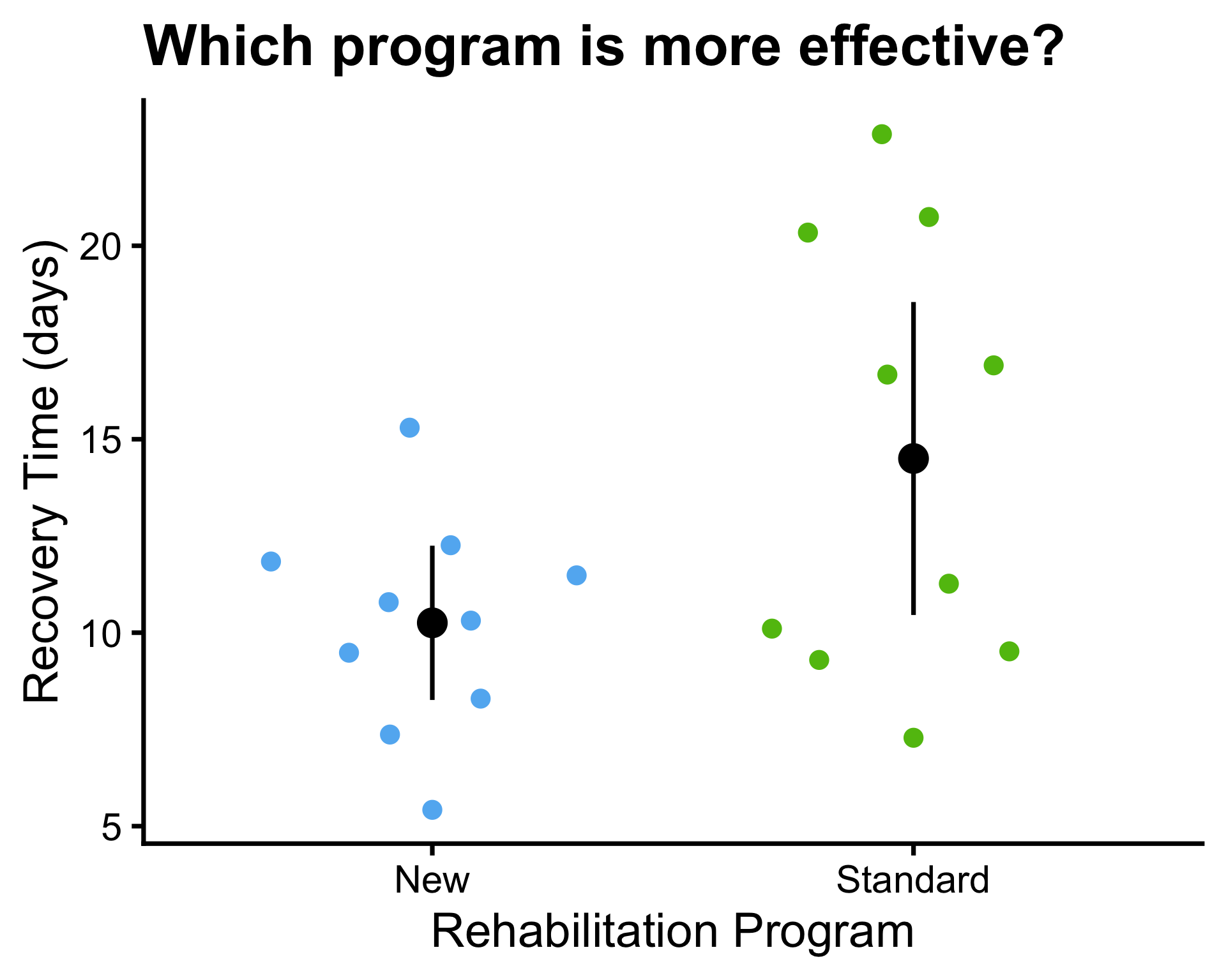
  • \(\mu_1 = 10\) and \(\mu_2 = 14\)
  • \(\bar{x}_1 = 10.3\) and \(\bar{x}_2 = 14.5\)
  • \(\sigma^2_1 = 4\) and \(\sigma^2_2 = 45\)
  • \(s_1^2 = 7.77\) and \(s_2^2 = 31.96\), \(s_p^2 = 19.86\)
  • \(n_1 = 10\) and \(n_2 = 10\)

P-values:

  • Known variance: \(P(Z \leq -1.9) = 0.0287\)
  • Unknown variance: \(P(t_{9} \leq -2.11) = 0.0320\)
  • Unknown equal variances: \(P(t_{18} \leq -2.11) = 0.0246\)
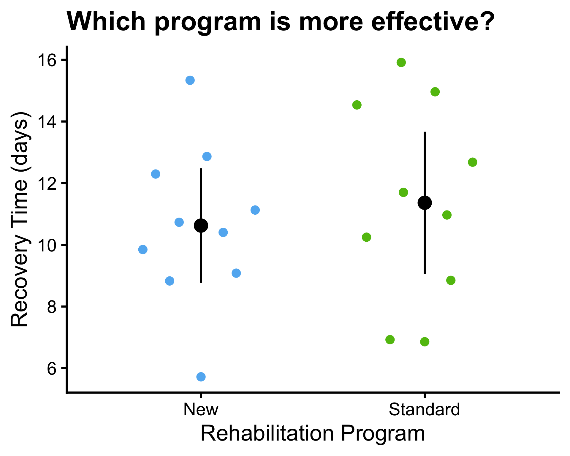
  • \(\mu_1 = 10\) and \(\mu_2 = 10\)
  • \(\bar{x}_1 = 10.6\) and \(\bar{x}_2 = 11.4\)
  • \(\sigma^2_1 = 9\) and \(\sigma^2_2 = 9\)
  • \(s_1^2 = 6.73\) and \(s_2^2 = 10.37\), \(s_p^2 = 8.55\)
  • \(n_1 = 10\) and \(n_2 = 10\)

P-values:

  • Known variance: \(P(Z \leq -0.6) = 0.2743\)
  • Unknown variance: \(P(t_{9} \leq -0.61) = 0.2785\)
  • Unknown equal variances: \(P(t_{18} \leq -0.61) = 0.2747\)
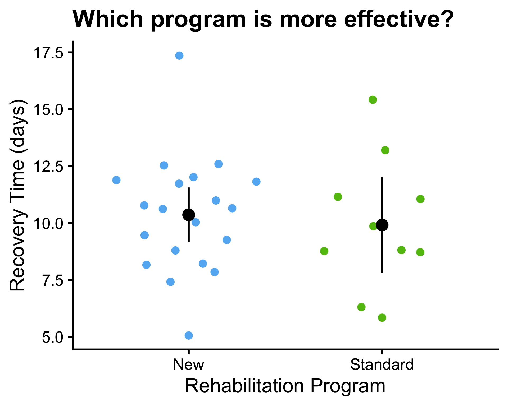
  • \(\mu_1 = 10\) and \(\mu_2 = 10\)
  • \(\bar{x}_1 = 10.4\) and \(\bar{x}_2 = 9.9\)
  • \(\sigma^2_1 = 9.89\) and \(\sigma^2_2 = 10\)
  • \(s_1^2 = 6.61\) and \(s_2^2 = 8.61\), \(s_p^2 = 7.25\)
  • \(n_1 = 20\) and \(n_2 = 10\)

P-values:

  • Known variance: \(P(Z \leq 0.41) = 0.6591\)
  • Unknown variance: \(P(t_{9} \leq 0.46) = 0.6718\)
  • Unknown equal variances: \(P(t_{28} \leq 0.48) = 0.6825\)

Case: Carbon dioxide and growth rate in algae

Growth rates of 14 unicellular alga Chlamydomonas after 1,000 generations of selection under High and Normal levels of carbon dioxide were examined.

Is there a difference in growth rates between the two carbon dioxide levels?

Two sample t-test using R

Assume that:

  • the growth rates are normally distributed, and
  • the samples within and between the two carbon dioxide levels are independent.

Note that:

  • When var.equal = FALSE, the two sample t-test uses the Welch-Satterthwaite approximation for the degrees of freedom (derivation out of scope for this course).
  • When var.equal = TRUE, the two sample t-test assumes that the population variances are equal and uses the pooled variance estimator.

Summary

scroll

\(H_0: \mu_1 = \mu_2\)

  • Observe \(n_1\) samples with sample mean \(\bar{X}_1\) from population 1 with mean \(\mu_1\).
  • Observe \(n_2\) samples with sample mean \(\bar{X}_2\) from population 2 with mean \(\mu_2\).
  • Samples from populations 1 and 2 should be independent.
  • Both populations are normally distributed or sample sizes \(n_1\) and \(n_2\) are sufficiently large.

Test statistic under \(H_0\)

Variances known

\[Z = \dfrac{\bar{X}_{1} - \bar{X}_{2}}{\sqrt{\frac{\sigma_{1}^2}{n_{1}} + \frac{\sigma_{2}^2}{n_{2}}}} \sim N(0, 1)\]

Variances unknown

\[T = \dfrac{\bar{X}_{1} - \bar{X}_{2}}{\sqrt{\frac{s_{1}^2}{n_{1}} + \frac{s_{2}^2}{n_{2}}}} \sim t_{\text{df}}\]

where

  • \(\text{df} = \min(n_{1}, n_{2}) - 1\) if variances cannot not be assumed to be equal and
  • \(\text{df} = n_{1} + n_{2} - 2\) if variances are assumed to be equal and \(s^2_1 = s^2_2 = s^2_p\).
  • \(s_p^2 = \dfrac{(n_{1} - 1)s_{1}^2 + (n_{2} - 1)s_{2}^2}{n_{1} + n_{2} - 2}\) is the pooled variance estimator.

Confidence interval for \(\mu_1 - \mu_2\)

Variances known

\[\bar{X}_{1} - \bar{X}_{2} \pm z_{\alpha / 2} \sqrt{\dfrac{\sigma_{1}^2}{n_{1}} + \dfrac{\sigma_{2}^2}{n_{2}}}\]

Variances unknown

\[\bar{X}_{1} - \bar{X}_{2} \pm t_{\text{df}, \alpha / 2} \sqrt{\dfrac{s_{1}^2}{n_{1}} + \dfrac{s_{2}^2}{n_{2}}}\]

P-value:

Variances known

\(H_A\) P-value
\(H_A: \mu_1 \neq \mu_2\) \(P(|Z| \geq |z^*|)\)
\(H_A: \mu_1 > \mu_2\) \(P(Z \geq z^*)\)
\(H_A: \mu_1 < \mu_2\) \(P(Z \leq z^*)\)

Variances unknown

\(H_A\) P-value
\(H_A: \mu_1 \neq \mu_2\) \(P(|T| \geq |t^*|)\)
\(H_A: \mu_1 > \mu_2\) \(P(T \geq t^*)\)
\(H_A: \mu_1 < \mu_2\) \(P(T \leq t^*)\)

Comparing Two Population Proportions

Example: CPR study

There is a new blood thinner drug that is believed to improve the survival rate of patients who underwent cardiopulmonary resuscitation (CPR) for a heart attack. Does the new drug improve the survival rate?

  • An experiment was conducted where 90 patients who underwent CPR for a heart attack and were subsequently admitted to a hospital were randomly divided into:
    • the treatment group where they received the blood thinner or
    • the control group where they did not receive the blood thinner.
  • The outcome variable of interest was whether the patients survived for at least 24 hours.
Group Survived Died Total
Treatment 11 39 50
Control 14 26 40
Total 25 65 90
  • Let \(p_1\) and \(p_2\) be the population proportions of patients who survived in the treatment and control groups, respectively.
  • We are interested in \(p_1 - p_2\).

Sampling distribution of the difference in sample proportions

  • Let \(X_{1}\) be the number of patients who survived out of \(n_1\) patients in the treatment group.
  • Let \(X_{2}\) be the number of patients who survived out of \(n_2\) patients in the control group.
  • The sample proportions are \(\hat{p}_1 = X_1/n_1\) and \(\hat{p}_2 = X_2/n_2\)
  • An estimator for \(p_1 - p_2\) is \(\hat{p}_1 - \hat{p}_2\).
  • Provided that:
    • the samples are independent within and between the two groups, and
    • success-failure condition is satisfied for CLT:
      \(n_1\hat{p}_1 \geq 10\), \(n_1(1-\hat{p}_1) \geq 10\), \(n_2\hat{p}_2 \geq 10\), and \(n_2(1-\hat{p}_2) \geq 10\),

\[\class{highlight mark-yellow}{\hat{p}_1 - \hat{p}_2 \sim N\left(p_1 - p_2, \sqrt{\frac{p_1(1-p_1)}{n_1} + \frac{p_2(1-p_2)}{n_2}}\right)}\]

\(100(1-\alpha)\%\) confidence interval for \(p_1 - p_2\)

\[\class{highlight mark-yellow}{\hat{p}_{1} - \hat{p}_{2} \pm z_{\alpha / 2} \sqrt{\frac{\hat{p}_1(1-\hat{p}_1)}{n_{1}} + \frac{\hat{p}_2(1-\hat{p}_2)}{n_{2}}}}\]

Group Survived Died Total
Treatment 11 39 50
Control 14 26 40
Total 25 65 90
  • \(\hat{p}_1 = 11/50 = 0.22\) and \(\hat{p}_2 = 14/40 = 0.35\)
  • We have \(n_1\hat{p}_1 = 11\), \(n_1(1-\hat{p}_1) = 39\), \(n_2\hat{p}_2 = 14\), and \(n_2(1-\hat{p}_2) = 26\), so the success-failure condition is satisfied.
  • This is a randomized experiment, so we can assume samples are independent within and between the two groups.

A 90% confidence interval for \(p_1 - p_2\) is given by:

\[\frac{11}{50} - \frac{14}{40} \pm z_{0.05} \sqrt{\frac{\frac{11}{50}(1-\frac{11}{50})}{50} + \frac{\frac{14}{40}(1-\frac{14}{40})}{40}} = (-0.2871, 0.0271).\]

where \(z_{0.05} \approx 1.645\).

Hypothesis testing for comparing two population proportions

\(H_0: p_1 = p_2\)

\[\class{highlight mark-yellow}{Z = \dfrac{\hat{p}_{1} - \hat{p}_{2}}{\sqrt{\hat{p}_{p}(1-\hat{p}_{p})(\frac{1}{n_{1}} + \frac{1}{n_{2}})}}} \sim N(0, 1) \text{ under } H_0\]

where \(\hat{p}_p = \dfrac{X_1 + X_2}{n_1 + n_2}\) is the pooled sample proportion.

  • \(H_A: p_1 < p_2\) \(\rightarrow\) P-value \(= P(Z \leq z^*)\)
  • \(H_A: p_1 > p_2\) \(\rightarrow\) P-value \(= P(Z \geq z^*)\)
  • \(H_A: p_1 \neq p_2\) \(\rightarrow\) P-value \(= 2P(Z \geq |z^*|)\)

where \(z^* = \dfrac{\frac{x_1}{n_1} - \frac{x_2}{n_2}}{\sqrt{\frac{x_1 + x_2}{n_1 + n_2}\left(1-\frac{x_1 + x_2}{n_1 + n_2}\right)\left(\frac{1}{n_{1}} + \frac{1}{n_{2}}\right)}}\).

\[\begin{align*} z^* &= \dfrac{\frac{11}{50} - \frac{14}{40}}{\sqrt{\frac{11 + 14}{50 + 40}\left(1-\frac{11 + 14}{50 + 40}\right)\left(\frac{1}{50} + \frac{1}{40}\right)}}\\ &= -1.37 \end{align*}\]

P-value \(= P(Z \geq -1.37) \approx 0.9147\).

Since P-value \(> 0.05\), there is no evidence to support the claim that the new drug improves the survival rate.

Example: Quadcopter rotor blade manufacturer

A quadcopter company is considering a new manufacturer for rotor blades. The new manufacturer would be more expensive, but they claim their higher-quality blades are more reliable, with at least 3% more blades passing inspection than their competitor. Is there evidence to support the claim?

  • The quality control engineer examines 1000 blades from each company.
  • She finds 958 blades pass inspection from the prospective supplier, and
  • 899 blades pass inspection from the current supplier.
  • Let \(p_1\) and \(p_2\) be the population proportions of blades that pass inspection for the prospective and current suppliers, respectively.
  • \(H_0: p_1 = p_2 + 0.03\) vs. \(H_A: p_1 > p_2 + 0.03\)
  • First, check the conditions:
    • the sample is not necessarily random, so we must assume the blades are independent within and between the two groups, and
    • the success-failure condition is satisfied for each company.
  • \(H_0\) is not \(p_1 = p_2\), so we cannot use the pooled sample proportion.
  • \(z^* = \dfrac{(0.958 - 0.899) - \class{highlight mark-green}{0.03}}{\sqrt{\class{highlight mark-green}{\frac{0.958(1 - 0.958)}{1000} + \frac{0.899(1 - 0.899)}{1000}}}} \approx 2.53\)
  • P-value \(= P(Z \geq 2.53) \approx 0.0057 < 0.05 \rightarrow\) there is evidence to support that the new manufacturer has at least 3% more blades that pass inspection.

Summary

\(H_0: p_1 = p_2\)

  • Observe \(n_1\) samples with \(X_1\) successes from population 1 with probability of success \(p_1\).
  • Observe \(n_2\) samples with \(X_2\) successes from population 2 with probability of success \(p_2\).
  • Samples from populations 1 and 2 should be independent.
  • Success-failture condition should be satisfied:

\[n_1\hat{p}_1 \geq 10, n_1(1-\hat{p}_1) \geq 10, n_2\hat{p}_2 \geq 10\text{, and }n_2(1-\hat{p}_2) \geq 10\]

Confidence interval for \(\mu_1 - \mu_2\)

\[\hat{p}_{1} - \hat{p}_{2} \pm z_{\alpha / 2} \sqrt{\frac{\hat{p}_1(1-\hat{p}_1)}{n_{1}} + \frac{\hat{p}_2(1-\hat{p}_2)}{n_{2}}}\]

\(\hat{p}_1 = \dfrac{X_1}{n_1}\), \(\hat{p}_2 = \dfrac{X_2}{n_2}\) and \(\hat{p}_p = \dfrac{X_1 + X_2}{n_1 + n_2}\)

Test statistic under \(H_0: p_1 = p_2\)

\[Z = \dfrac{\hat{p}_{1} - \hat{p}_{2}}{\sqrt{\hat{p}_{p}(1-\hat{p}_{p})(\frac{1}{n_{1}} + \frac{1}{n_{2}})}} \sim N(0, 1)\]

P-value:

\(H_A\) P-value
\(H_A: p_1 \neq p_2\) \(P(|Z| \geq |z^*|)\)
\(H_A: p_1 > p_2\) \(P(Z \geq z^*)\)
\(H_A: p_1 < p_2\) \(P(Z \leq z^*)\)

Paired Samples

Independent vs. paired samples

  • Are men earning more than women?
  • A random sample of men and women are selected and their incomes are recorded.
  • This is an example of independent samples.
  • Are husbands earning more than their wives?
  • A random sample of husbands and their wives are selected and their incomes are recorded.
  • This is an example of paired samples.
  • Whether you should collect independent samples or paired samples will be determined by your research question.

Example: textbook prices

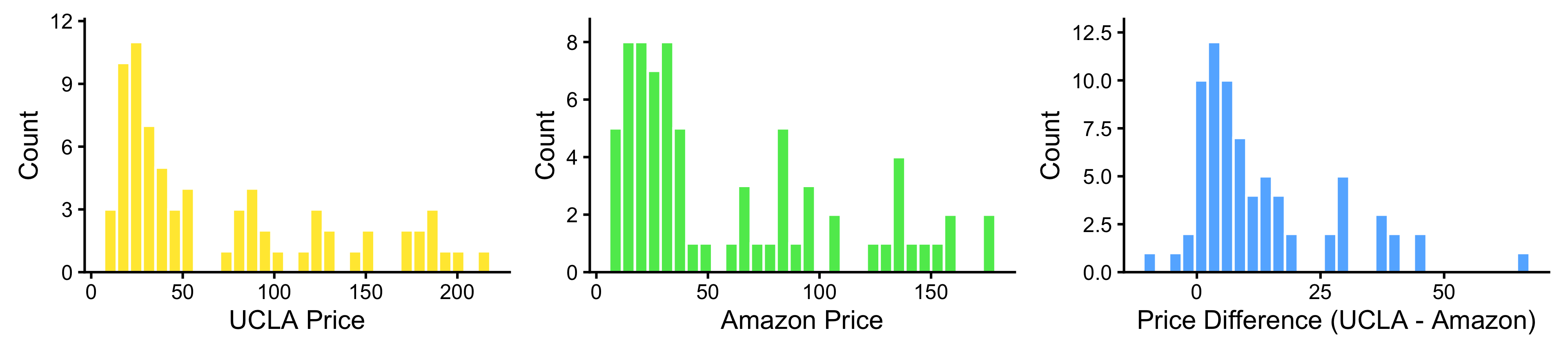
Are the prices of textbooks on Amazon close to ones in the UCLA bookstore?

73 textbooks were identified as required for UCLA courses.

The price of each textbook on Amazon and the university bookstore was recorded.

Course ISBN
Price (USD)
UCLA Amazon Difference
C139 978-0520224759 18.75 20.21 -1.46
104 978-0470419977 174.00 143.75 30.25
C170 978-0803272620 27.67 27.95 -0.28
M422 978-0761918479 88.42 97.95 -9.53
127B 978-0324828641 214.50 173.56 40.94
10 978-0195181234 24.70 16.47 8.23
M104D 978-1412969666 89.71 85.45 4.26
M132B 978-0205753383 55.13 42.68 12.45
M104C 978-0582276024 16.00 11.67 4.33
124 978-0078136634 183.75 145.40 38.35

Paired data

  • The price of the same textbook on Amazon and the university bookstore are paired data.
  • Let:
    • \(X_{1i}\) be the price of the \(i\)-th textbook at the university bookstore,
    • \(X_{2i}\) be the price of the \(i\)-th textbook on Amazon, and
    • \(X_{di} = X_{1i} - X_{2i}\) be the price difference for the \(i\)-th textbook.
  • For paired data, we are often interested in the difference between the two responses, \(D_i\), effectively reducing the problem to a one-sample.

Inference for paired data

  • Suppose that
    • \(\mu_1\) is the mean price of the textbooks at the university bookstore,
    • \(\mu_2\) is the mean price of the textbooks on Amazon, and
    • \(\mu_d = \mu_1 - \mu_2\) is the mean price difference between the two sources.
  • A \(100(1-\alpha)\%\) confidence interval for \(\mu_d\) is given by: \[\class{highlight mark-yellow}{\bar{X}_d \pm t_{n-1, \alpha / 2} \frac{s_d}{\sqrt{n}}}\] where
    • \(\bar{X}_d\) is the sample mean of the differences, and
    • \(s_d\) is the sample standard deviation of the differences, and
    • \(n\) is the number of pairs.
Source n Mean Price Standard Deviation
UCLA 73 72.22 59.66
Amazon 73 59.46 49.00
Difference 73 12.76 14.26
  • Assume that the price differences are independent and normally distributed.
  • A 95% confidence interval for \(\mu_d\) is given by:

\(12.76 \pm t_{72, 0.025} \times \dfrac{14.26}{\sqrt{73}}\) \(\approx\) \((9.44, 16.09).\)

  • Therefore we are 95% confident that the mean price difference between the university bookstore and Amazon is between $9.44 and $16.09.

Hypothesis testing for paired data

\(H_0: \mu_d = 0 \text{ vs. } H_A: \mu_d \neq 0\)

\[\class{highlight mark-yellow}{T = \dfrac{\bar{X}_d}{s_d / \sqrt{n}}} \sim t_{n-1} \text{ under } H_0\]

  • P-value \(= 2P(T \geq |t^*|)\) where \(t^*\) is the observed value of the test statistic.
  • \(t^* = \dfrac{12.76}{14.26/\sqrt{73}} \approx 7.65\)

  • P-value \(= 2P(T \geq 7.65) \approx 0.0000\).

  • Since P-value \(< 0.05\), there is evidence to support that the prices of textbooks on Amazon are significantly different from the ones in the UCLA bookstore.

Summary

scroll

\(H_0: \mu_d = 0\)

  • For paired data, we are often interested in the difference between the two responses, effectively reducing the problem to a one-sample.
  • Observe a pair of \(n\) samples with sample mean difference \(\bar{X}_d\) and sample standard deviation of the differences \(s_d\) from the population with mean difference \(\mu_d\) and standard deviation of the differences \(\sigma_d\).

Confidence interval for \(\mu_d\)

Variance known

\[\bar{X}_d \pm z_{\alpha / 2} \frac{\sigma_d}{\sqrt{n}}\]

Variance unknown

\[\bar{X}_d \pm t_{n - 1, \alpha / 2} \frac{s_d}{\sqrt{n}}\]

P-value

Variance known

\(Z = \dfrac{\bar{X}_d}{\sigma_d / \sqrt{n}} \sim N(0, 1)\) under \(H_0\).

\(H_A\) P-value
\(H_A: \mu_d \neq 0\) \(P(|Z| \geq |z^*|)\)
\(H_A: \mu_d > 0\) \(P(Z \geq z^*)\)
\(H_A: \mu_d < 0\) \(P(Z \leq z^*)\)

Variance unknown

\(T = \dfrac{\bar{X}_d}{s_d / \sqrt{n}} \sim t_{n - 1}\) under \(H_0\).

\(H_A\) P-value
\(H_A: \mu_d \neq 0\) \(P(|T| \geq |t^*|)\)
\(H_A: \mu_d > 0\) \(P(T \geq t^*)\)
\(H_A: \mu_d < 0\) \(P(T \leq t^*)\)