Comparing two population means

STAT1003 – Statistical Techniques

Dr. Emi Tanaka

Australian National University

These slides are best viewed on a modern browser like Google Chrome on a desktop or laptop. Some interactive components may require some time to fully load.

Example: rehabilitation program

  • A hospital is comparing two rehabilitation programs (Standard and New) for patients recovering from knee surgery.
  • Patients are randomly assigned to one of the two programs.
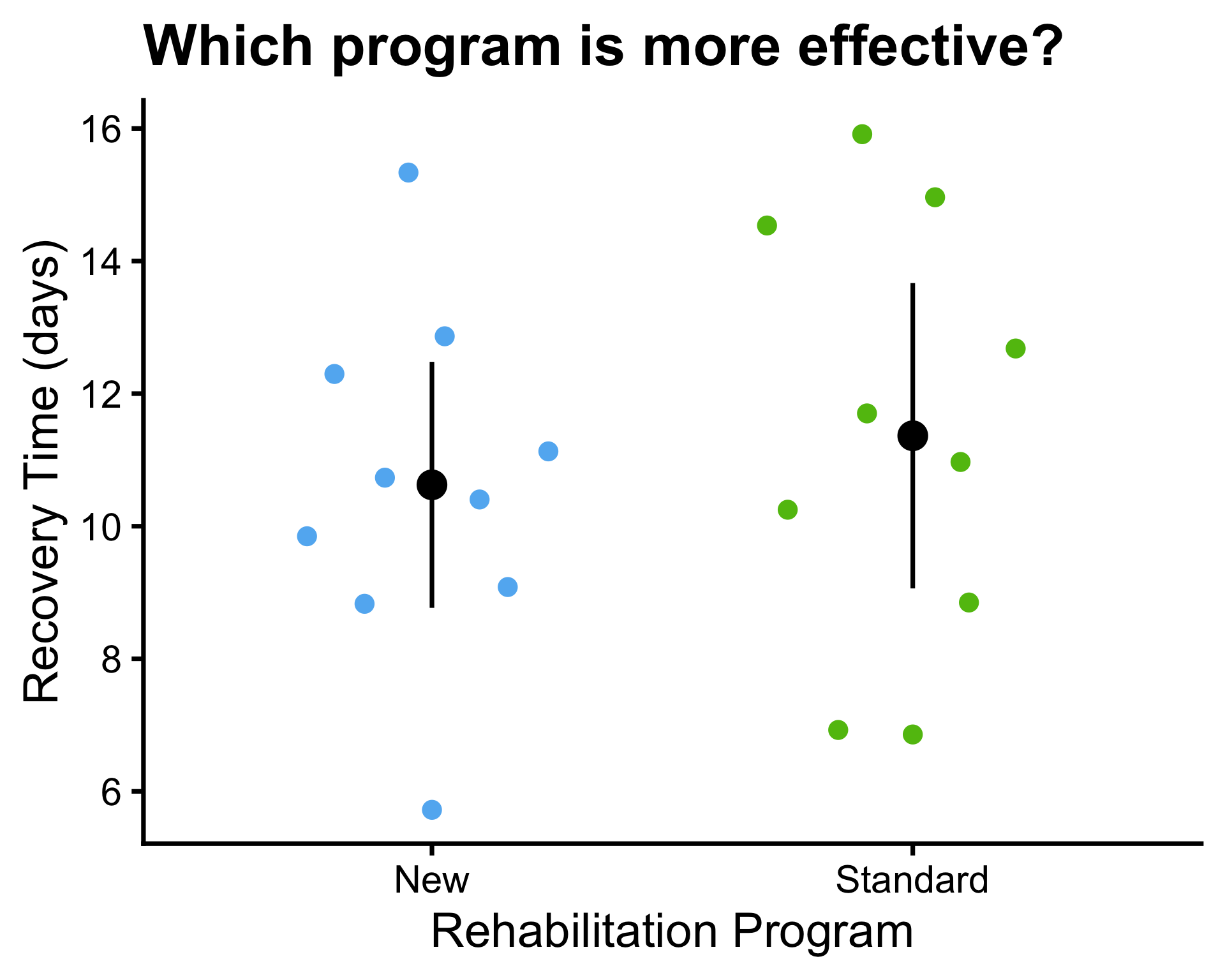
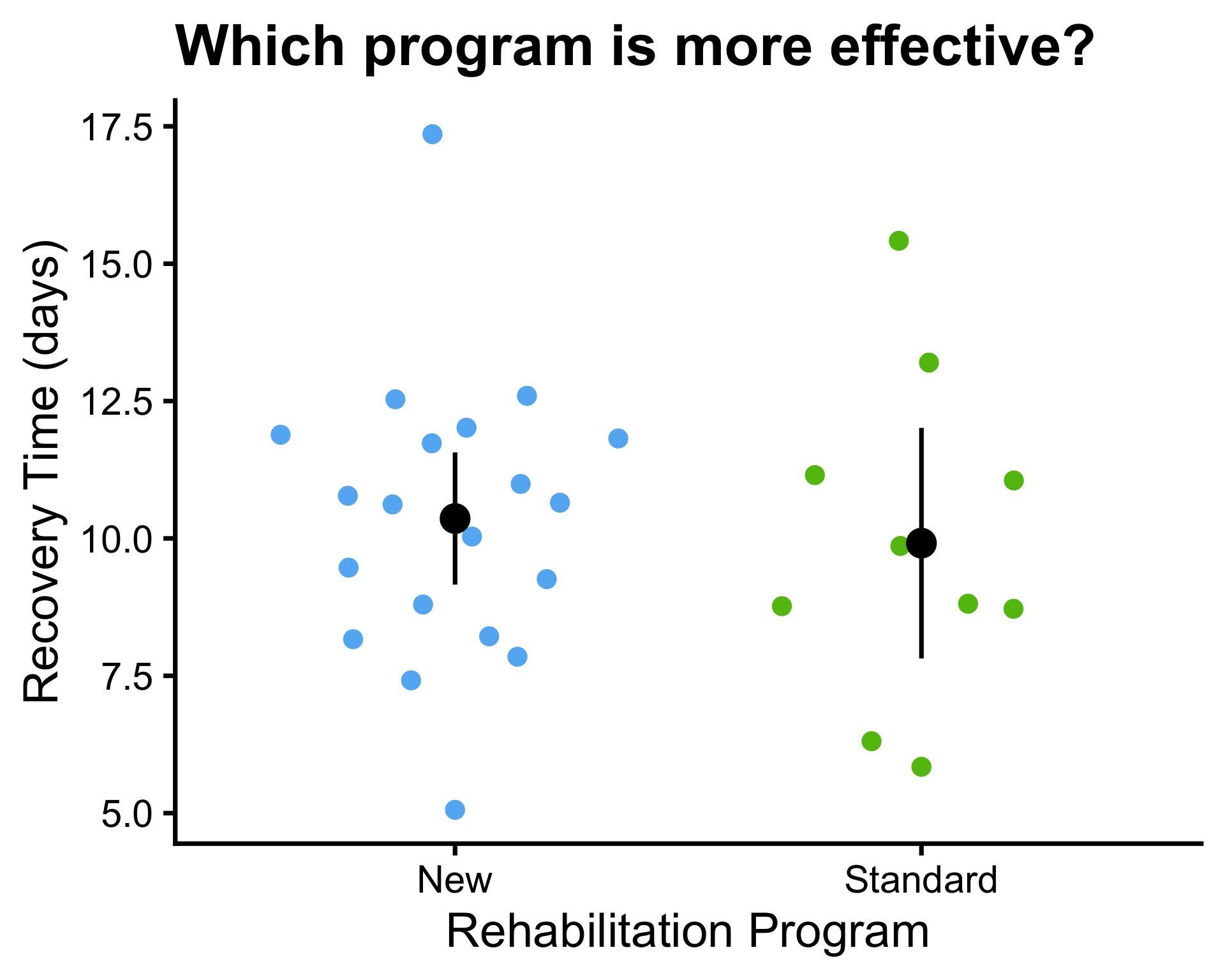
  • The recovery time (in days) until patients can walk unassisted is recorded for each patient.

Is the new program more effective than the standard program in reducing recovery time?

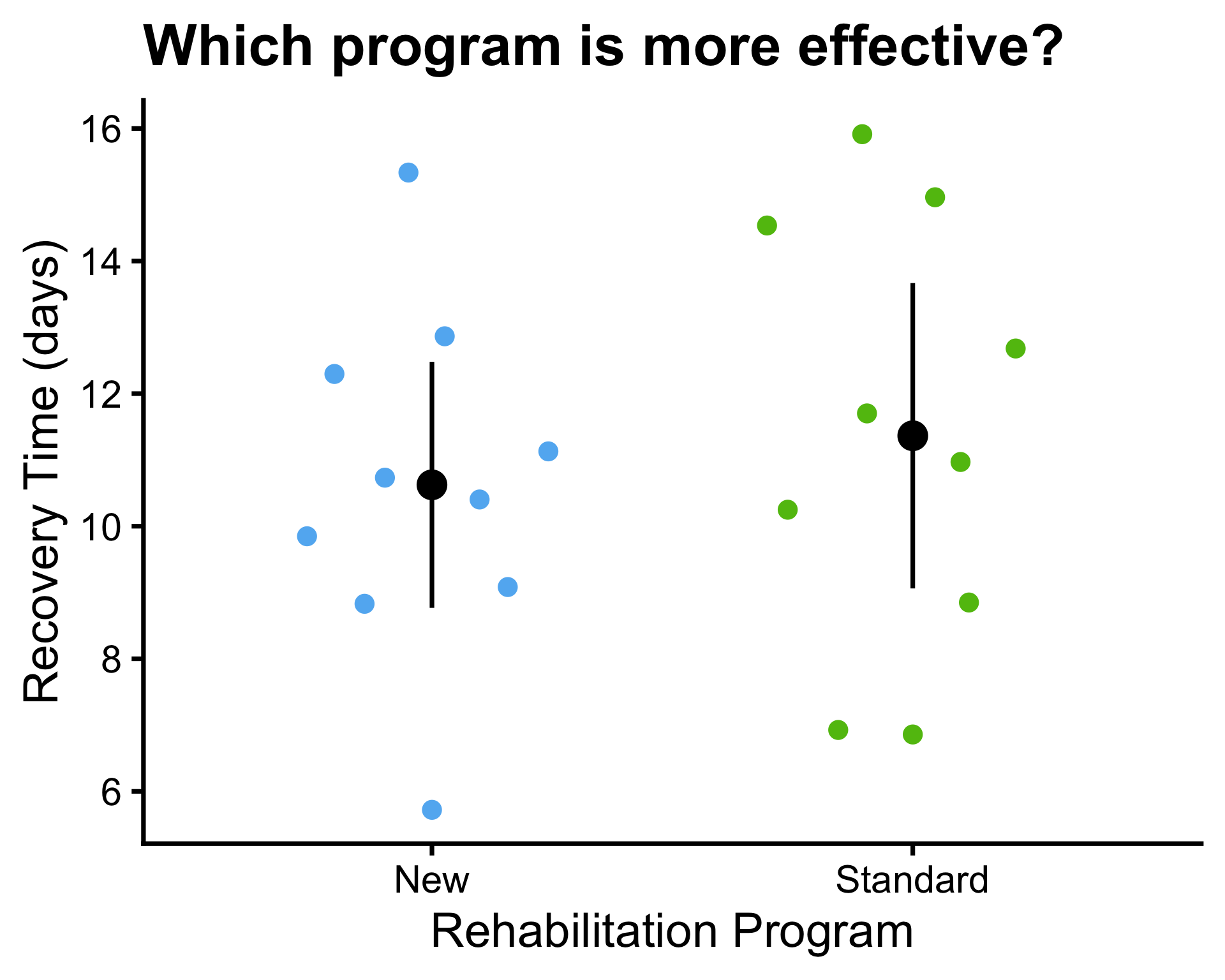
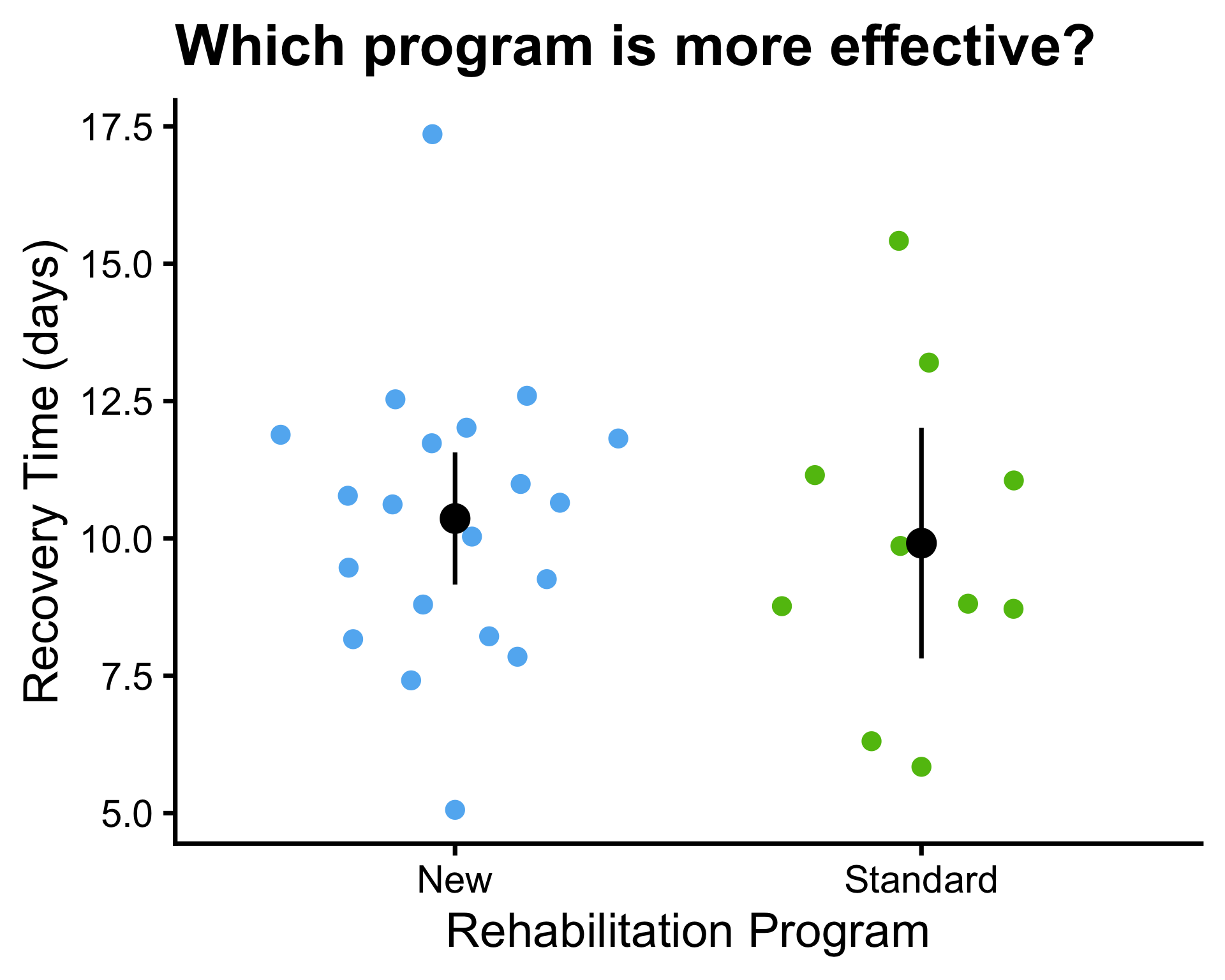
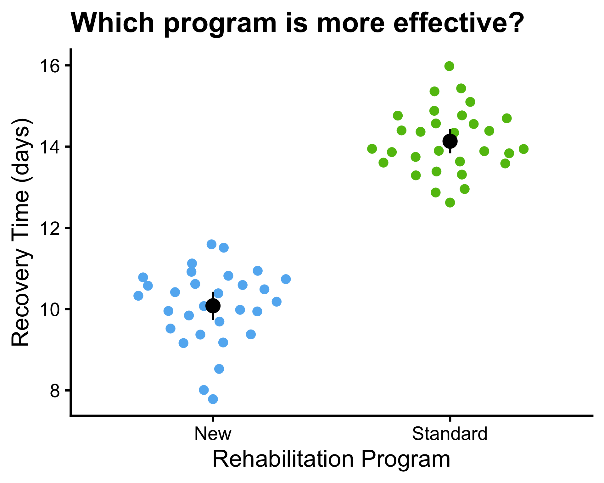
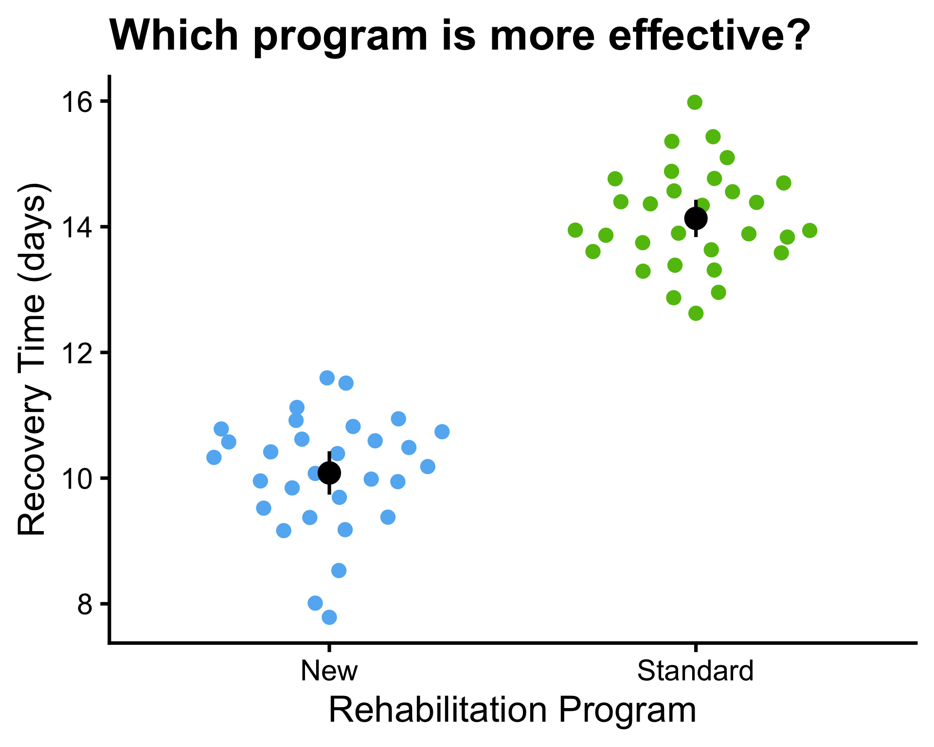
  • A beeswarm plot is a type of scatter plot that shows the distribution of a continuous variable across different groups.
  • In a beeswarm plot, the data points are arranged in a way that minimizes overlap, allowing for a clearer visualization of the distribution and density of the data within each group.
Example: hypotheses for comparing two means

Is the new program more effective than the standard program in reducing recovery time?

  • Let \(\mu_{1}\) be the mean recovery time for patients in the new rehabilitation program.
  • Let \(\mu_{2}\) be the mean recovery time for patients in the standard rehabilitation program.
  • What parameter is of interest? \(\mu_{1} - \mu_{2}\).
  • \(H_0: \mu_{1} - \mu_{2} = 0\) vs. \(H_A: \mu_{1} - \mu_{2} < 0\) (note: lower recovery time is better)
    \[\rightarrow \class{highlight mark-yellow}{H_0: \mu_{1} = \mu_{2}\quad\text{ vs. }\quad H_A: \mu_{1} < \mu_{2}}\]
  • What is a reasonable point estimator (and therefore test statistic) for \(\mu_{1} - \mu_{2}\)? \(\bar{X}_{1} - \bar{X}_{2}\).
  • What is sampling distribution of this point estimator?
  • If the samples are independent (between and within groups) and sample size is large enough (or the populations are normally distributed), then \[\class{highlight mark-yellow}{\bar{X}_{1} - \bar{X}_{2}\overset{\text{approx.}}{\sim} N\left(\mu_{1} - \mu_{2}, \frac{\sigma_1^2}{n_1} + \frac{\sigma_2^2}{n_2}\right)}\] where \(\sigma_j^2\) and \(n_j\) are the population variance and sample size for group \(j \in \{1, 2\}\), respectively.

Test statistic and its distribution

\[Z = \dfrac{(\bar{X}_{1} - \bar{X}_{2}) - (\mu_{1} - \mu_{2})}{\sqrt{\dfrac{\sigma_{1}^2}{n_{1}} + \dfrac{\sigma_{2}^2}{n_{2}}}}\]

\(Z \sim N(0, 1)\) under \(H_0: \mu_{1} = \mu_{2}\).

\[T = \dfrac{(\bar{X}_{1} - \bar{X}_{2}) - (\mu_{1} - \mu_{2})}{\sqrt{\dfrac{s_{1}^2}{n_{1}} + \dfrac{s_{2}^2}{n_{2}}}}\]

\(T \sim t_{\class{highlight mark-yellow}{\min(n_{1}, n_{2}) - 1}}\) under \(H_0: \mu_{1} = \mu_{2}\).

  • Note that the degrees of freedom above is a conservative estimate.
  • The degrees of freedom can be calculated using a more complex formula (Welch-Satterthwaite equation), but we will not cover its derivation in this course.

Special case: equal variances

  • Suppose we have reason to believe that the population variances are equal, i.e., \(\sigma_{1}^2 = \sigma_{2}^2 = \sigma^2\).
  • \(\sigma^2\) can be estimated by pooling the sample variances from the two groups: \[\class{highlight mark-yellow}{s_p^2 = \dfrac{(n_{1} - 1)s_{1}^2 + (n_{2} - 1)s_{2}^2}{n_{1} + n_{2} - 2}} = \frac{\sum_{i=1}^{n_1}(x_{i,1} - \bar{x}_{1})^2 + \sum_{i=1}^{n_2}(x_{i,2} - \bar{x}_{2})^2}{n_{1} + n_{2} - 2}\]

\[T = \dfrac{(\bar{X}_{1} - \bar{X}_{2}) - (\mu_{1} - \mu_{2})}{\sqrt{\class{highlight mark-yellow}{s_p^2}\left(\dfrac{1}{n_{1}} + \dfrac{1}{n_{2}}\right)}}\]

\(T \sim t_{\class{highlight mark-yellow}{n_{1} + n_{2} - 2}}\) under \(H_0: \mu_{1} = \mu_{2}\).

\(100(1-\alpha)\%\) confidence interval for \(\mu_{1} - \mu_{2}\)

\[\bar{X}_{1} - \bar{X}_{2} \pm z_{\alpha / 2} \sqrt{\dfrac{\sigma_{1}^2}{n_{1}} + \dfrac{\sigma_{2}^2}{n_{2}}}\]

\[\bar{X}_{1} - \bar{X}_{2} \pm t_{\text{df}, \alpha / 2} \sqrt{\dfrac{s_{1}^2}{n_{1}} + \dfrac{s_{2}^2}{n_{2}}}\]

where:

  • \(\text{df} = \min(n_{1}, n_{2}) - 1\) if variances cannot not be assumed to be equal
  • \(\text{df} = n_{1} + n_{2} - 2\) if variances are assumed to be equal and \(s^2_1 = s^2_2 = s^2_p\).

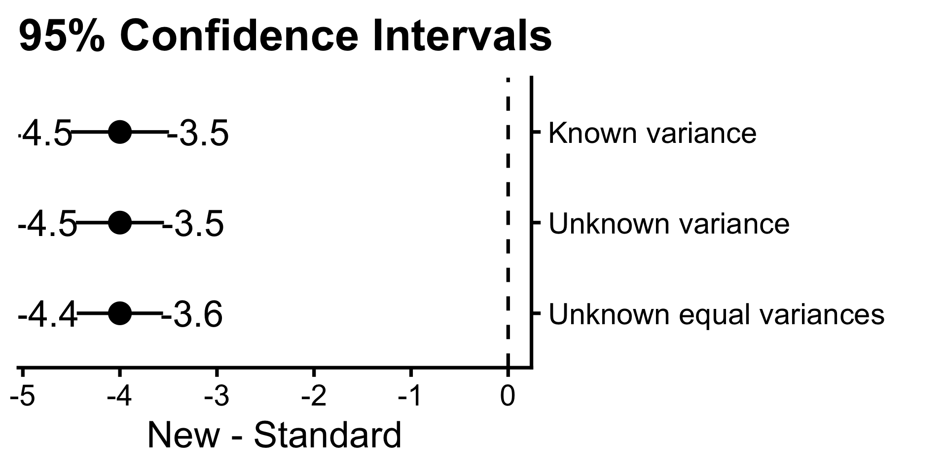
Example: 95% confidence interval

  • \(\mu_1 = 10\) and \(\mu_2 = 14\)
  • \(\bar{x}_1 = 10.1\) and \(\bar{x}_2 = 14.1\)
  • \(\sigma^2_1 = 1\) and \(\sigma^2_2 = 1\)
  • \(s_1^2 = 0.85\) and \(s_2^2 = 0.63\), \(s_p^2 = 0.74\)
  • \(n_1 = 30\) and \(n_2 = 30\)

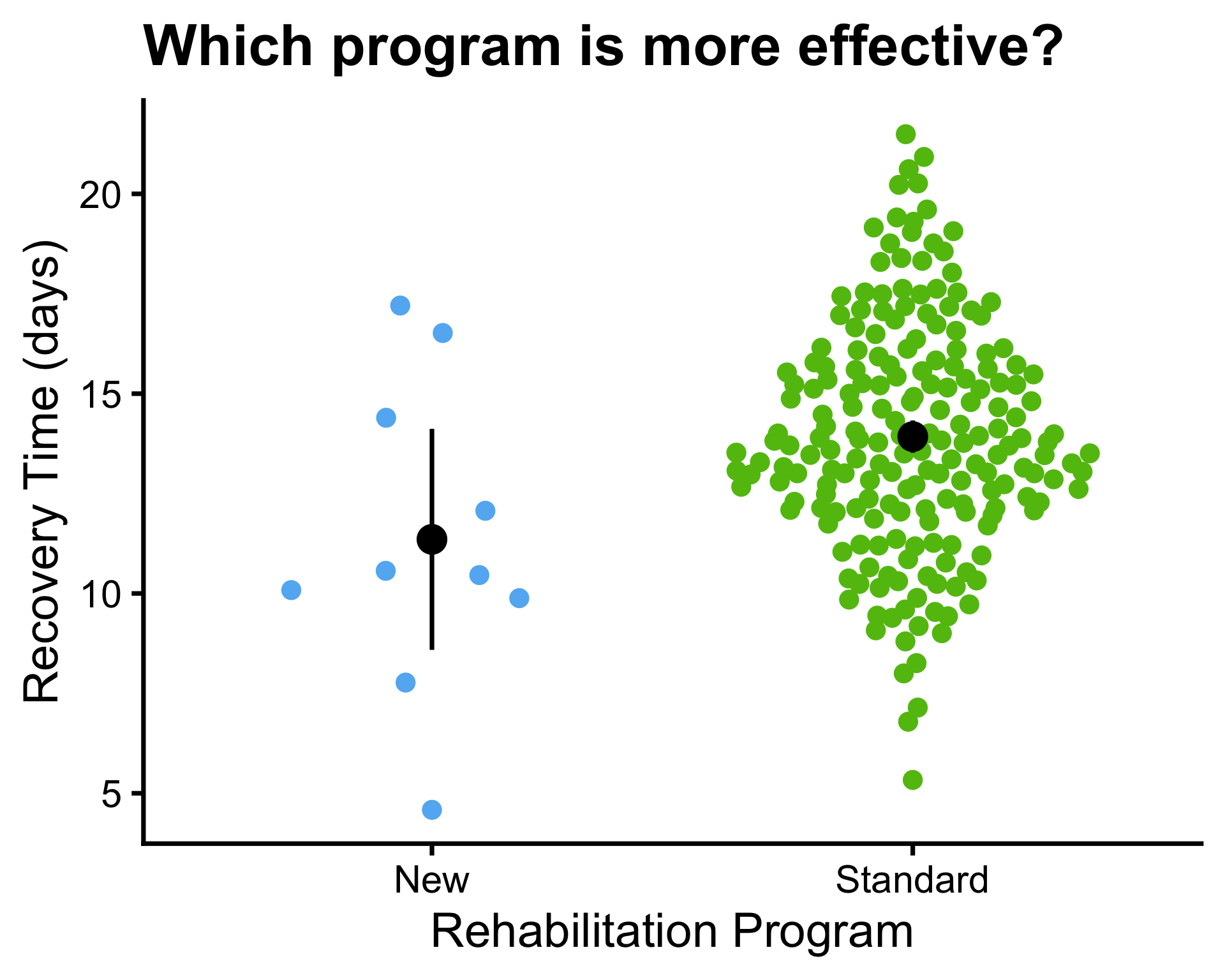
  • \(\mu_1 = 10\) and \(\mu_2 = 14\)
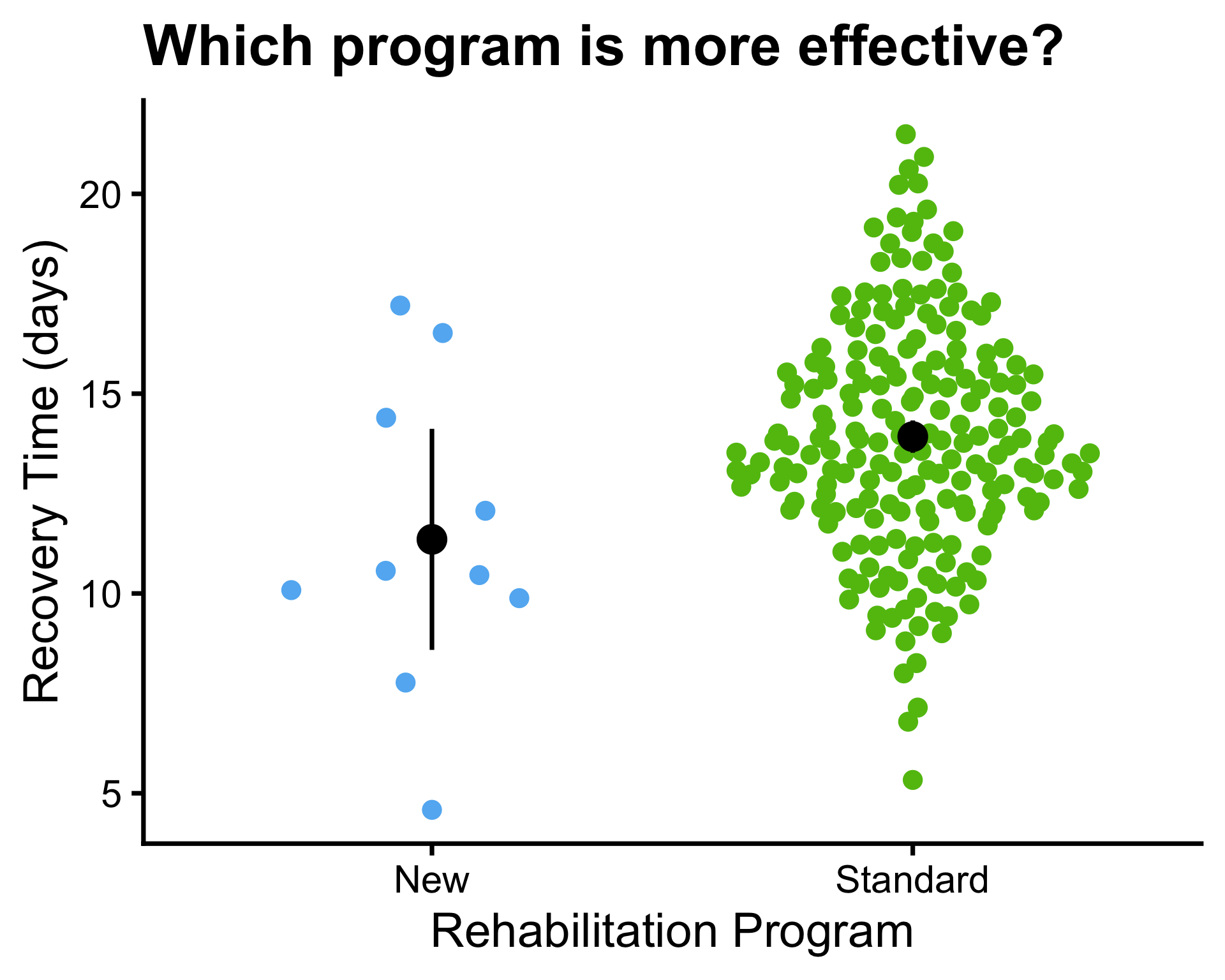
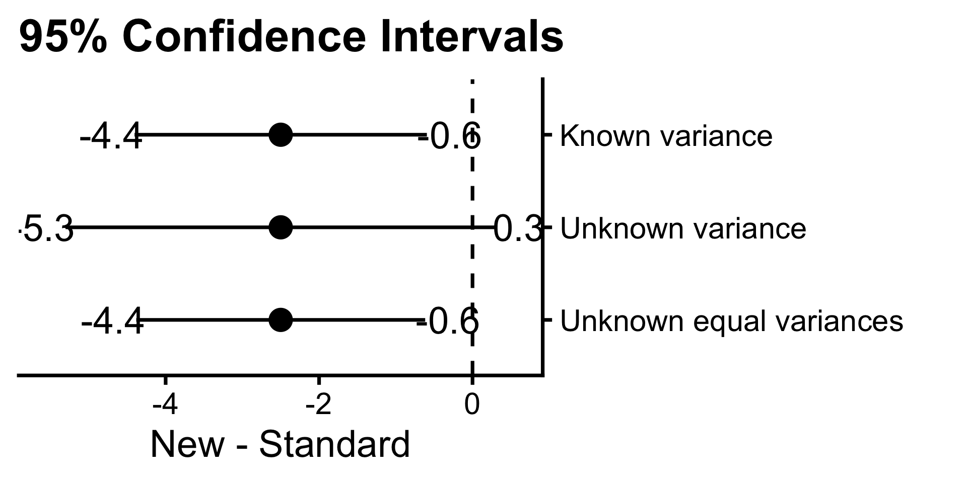
  • \(\bar{x}_1 = 11.4\) and \(\bar{x}_2 = 13.9\)
  • \(\sigma^2_1 = 9\) and \(\sigma^2_2 = 9\)
  • \(s_1^2 = 14.95\) and \(s_2^2 = 8.4\), \(s_p^2 = 8.69\)
  • \(n_1 = 10\) and \(n_2 = 200\)

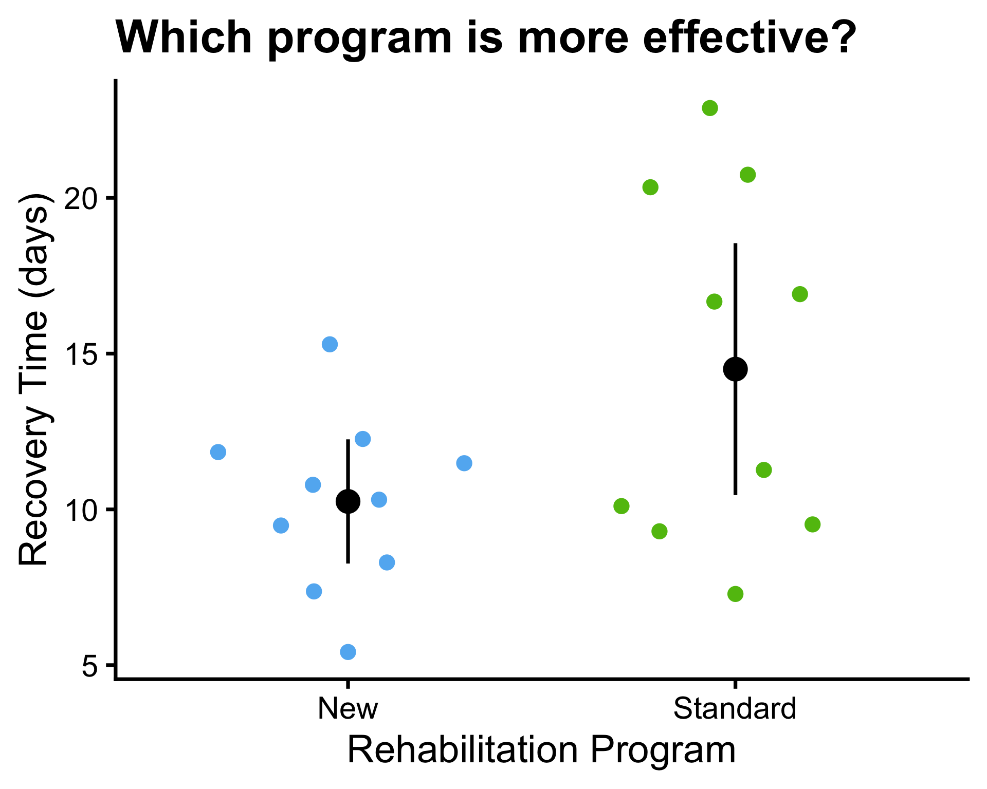
  • \(\mu_1 = 10\) and \(\mu_2 = 14\)
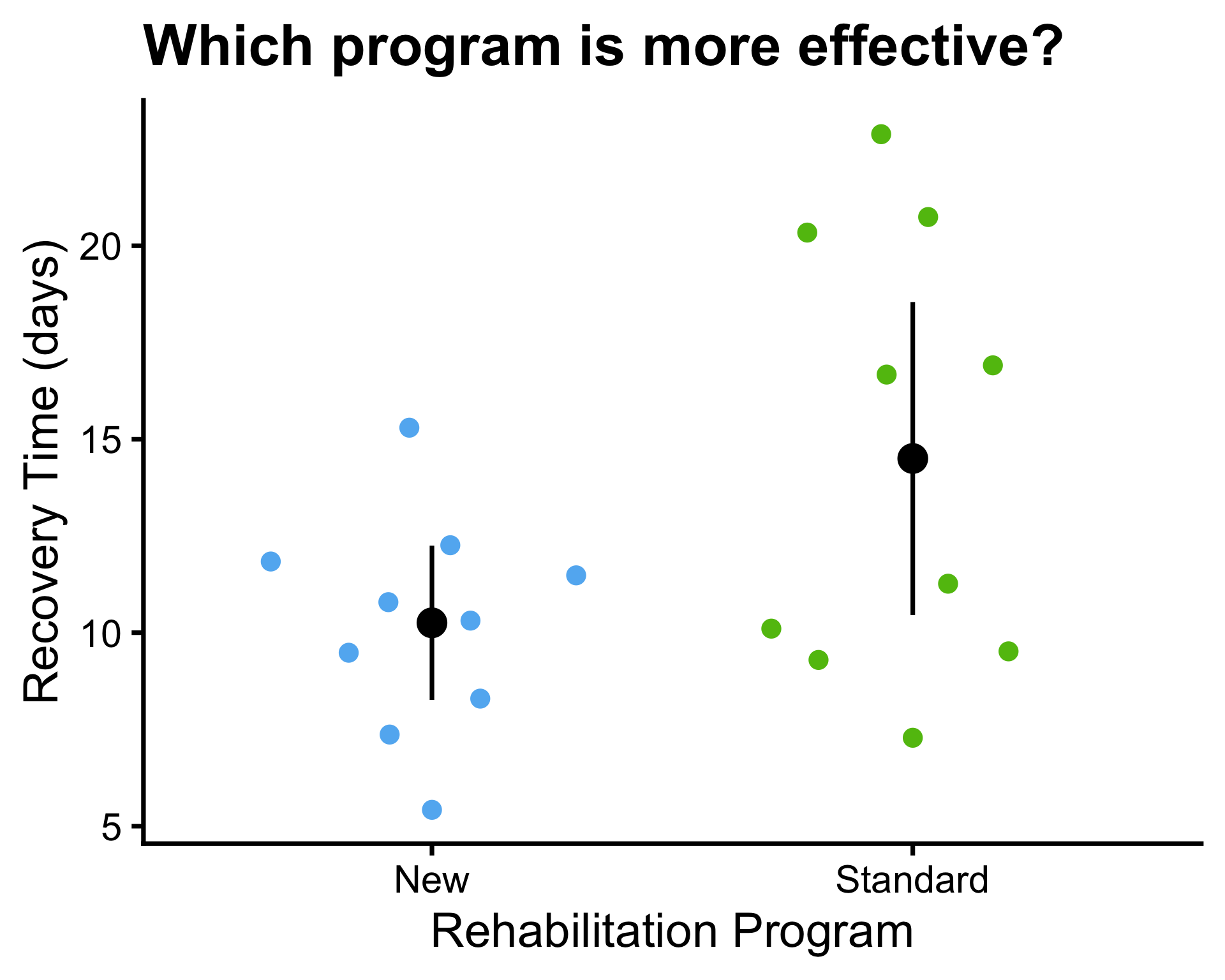
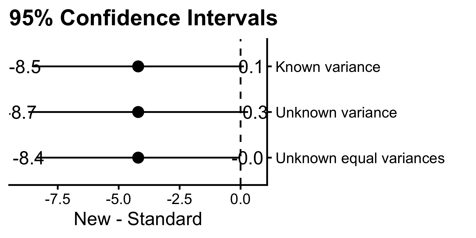
  • \(\bar{x}_1 = 10.3\) and \(\bar{x}_2 = 14.5\)
  • \(\sigma^2_1 = 4\) and \(\sigma^2_2 = 45\)
  • \(s_1^2 = 7.77\) and \(s_2^2 = 31.96\), \(s_p^2 = 19.86\)
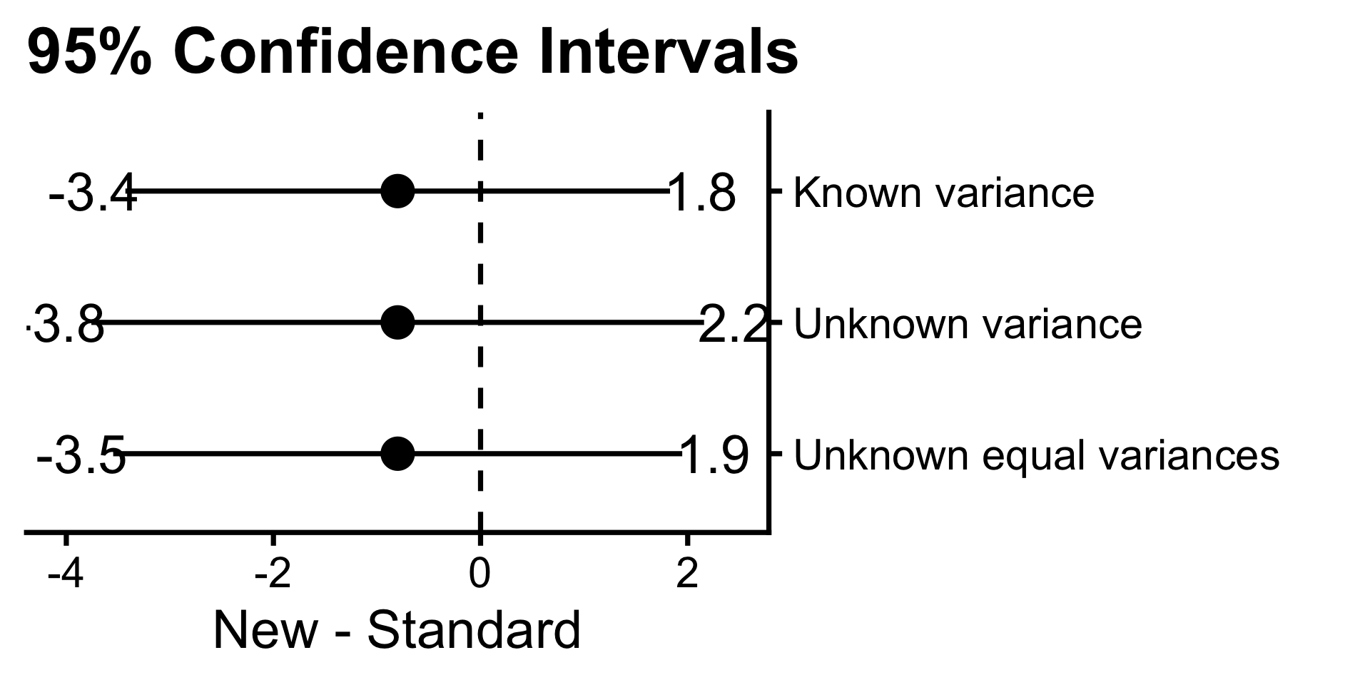
  • \(n_1 = 10\) and \(n_2 = 10\)

  • \(\mu_1 = 10\) and \(\mu_2 = 10\)
  • \(\bar{x}_1 = 10.6\) and \(\bar{x}_2 = 11.4\)
  • \(\sigma^2_1 = 9\) and \(\sigma^2_2 = 9\)
  • \(s_1^2 = 6.73\) and \(s_2^2 = 10.37\), \(s_p^2 = 8.55\)
  • \(n_1 = 10\) and \(n_2 = 10\)

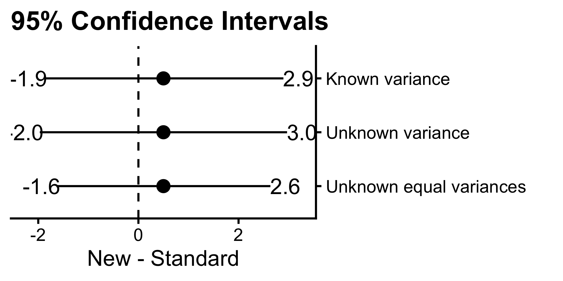
  • \(\mu_1 = 10\) and \(\mu_2 = 10\)
  • \(\bar{x}_1 = 10.4\) and \(\bar{x}_2 = 9.9\)
  • \(\sigma^2_1 = 9.89\) and \(\sigma^2_2 = 10\)
  • \(s_1^2 = 6.61\) and \(s_2^2 = 8.61\), \(s_p^2 = 7.25\)
  • \(n_1 = 20\) and \(n_2 = 10\)

Hypothesis testing for comparing two means

\(H_0: \mu_1 = \mu_2\)

\(z^* = \dfrac{\bar{x}_{1} - \bar{x}_{2}}{\sqrt{\dfrac{\sigma_1^2}{n_1} + \dfrac{\sigma_2^2}{n_2}}}\)

  • \(H_A: \mu_1 < \mu_2\)
    P-value \(= P(Z \leq z^*)\)
  • \(H_A: \mu_1 > \mu_2\)
    P-value \(= P(Z \geq z^*)\)
  • \(H_A: \mu_1 \neq \mu_2\)
    P-value \(= 2P(Z \geq |z^*|)\)

where \(Z \sim N(0, 1)\) under \(H_0\).

\(t^* = \dfrac{\bar{x}_{1} - \bar{x}_{2}}{\sqrt{\dfrac{s_1^2}{n_1} + \dfrac{s_2^2}{n_2}}}\)

  • \(H_A: \mu_1 < \mu_2\) \(\rightarrow\) P-value \(= P(T \leq t^*)\)
  • \(H_A: \mu_1 > \mu_2\) \(\rightarrow\) P-value \(= P(T \geq t^*)\)
  • \(H_A: \mu_1 \neq \mu_2\) \(\rightarrow\) P-value \(= 2P(T \geq |t^*|)\)

where

  • \(T \sim t_{\text{df}}\) under \(H_0\),
  • \(\text{df} = \min(n_{1}, n_{2}) - 1\) if variances cannot not be assumed to be equal, and
  • \(\text{df} = n_{1} + n_{2} - 2\) if variances are assumed to be equal and \(s^2_1 = s^2_2 = s^2_p\).

Example: p-values

  • \(\mu_1 = 10\) and \(\mu_2 = 14\)
  • \(\bar{x}_1 = 10.1\) and \(\bar{x}_2 = 14.1\)
  • \(\sigma^2_1 = 1\) and \(\sigma^2_2 = 1\)
  • \(s_1^2 = 0.85\) and \(s_2^2 = 0.63\), \(s_p^2 = 0.74\)
  • \(n_1 = 30\) and \(n_2 = 30\)

P-values:

  • Known variance: \(P(Z \leq -15.49) = 0.0000\)
  • Unknown variance: \(P(t_{29} \leq -18.01) = 0.0000\)
  • Unknown equal variances: \(P(t_{58} \leq -18.01) = 0.0000\)
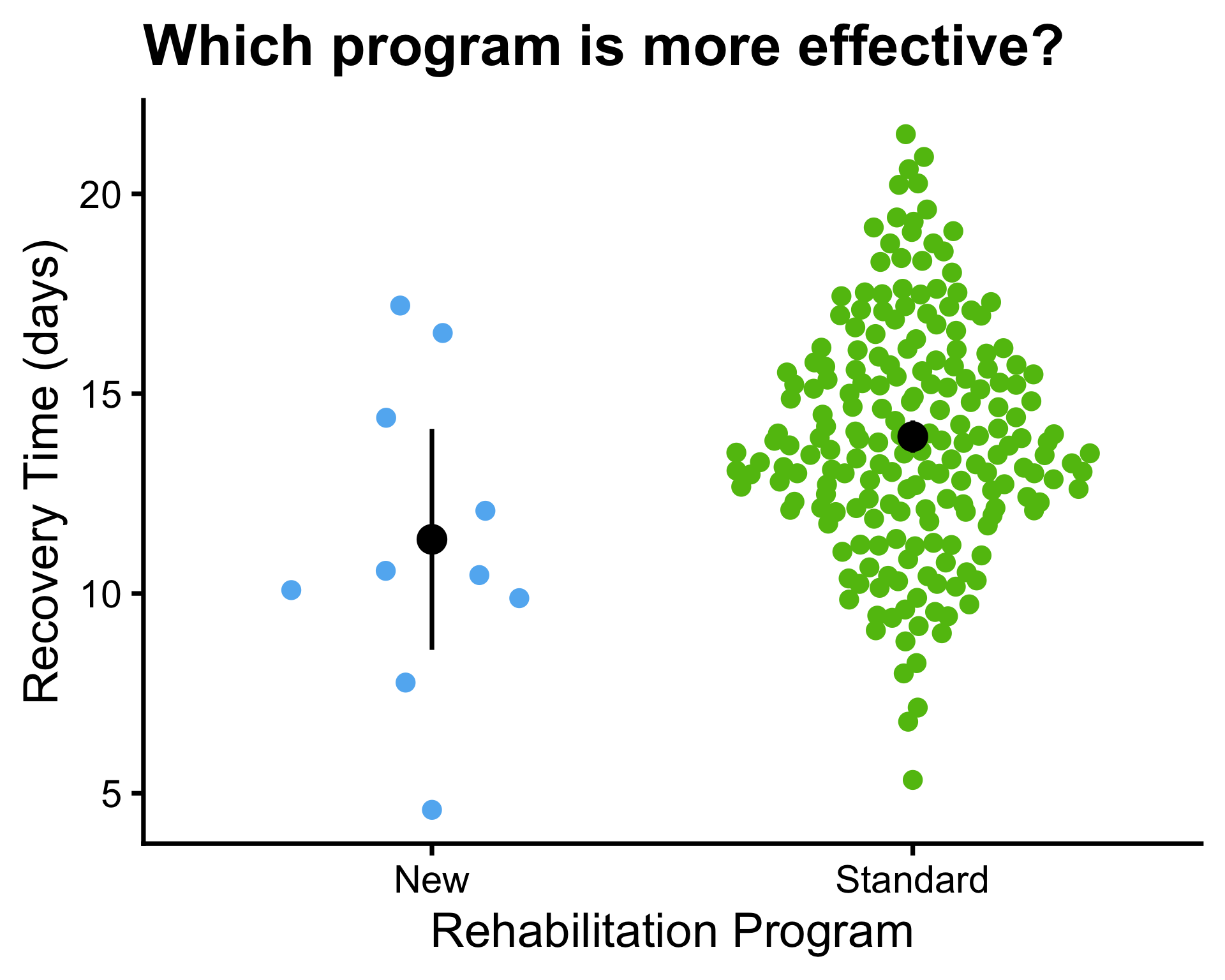
  • \(\mu_1 = 10\) and \(\mu_2 = 14\)
  • \(\bar{x}_1 = 11.4\) and \(\bar{x}_2 = 13.9\)
  • \(\sigma^2_1 = 9\) and \(\sigma^2_2 = 9\)
  • \(s_1^2 = 14.95\) and \(s_2^2 = 8.4\), \(s_p^2 = 8.69\)
  • \(n_1 = 10\) and \(n_2 = 200\)

P-values:

  • Known variance: \(P(Z \leq -2.57) = 0.0051\)
  • Unknown variance: \(P(t_{9} \leq -2.02) = 0.0371\)
  • Unknown equal variances: \(P(t_{208} \leq -2.62) = 0.0047\)
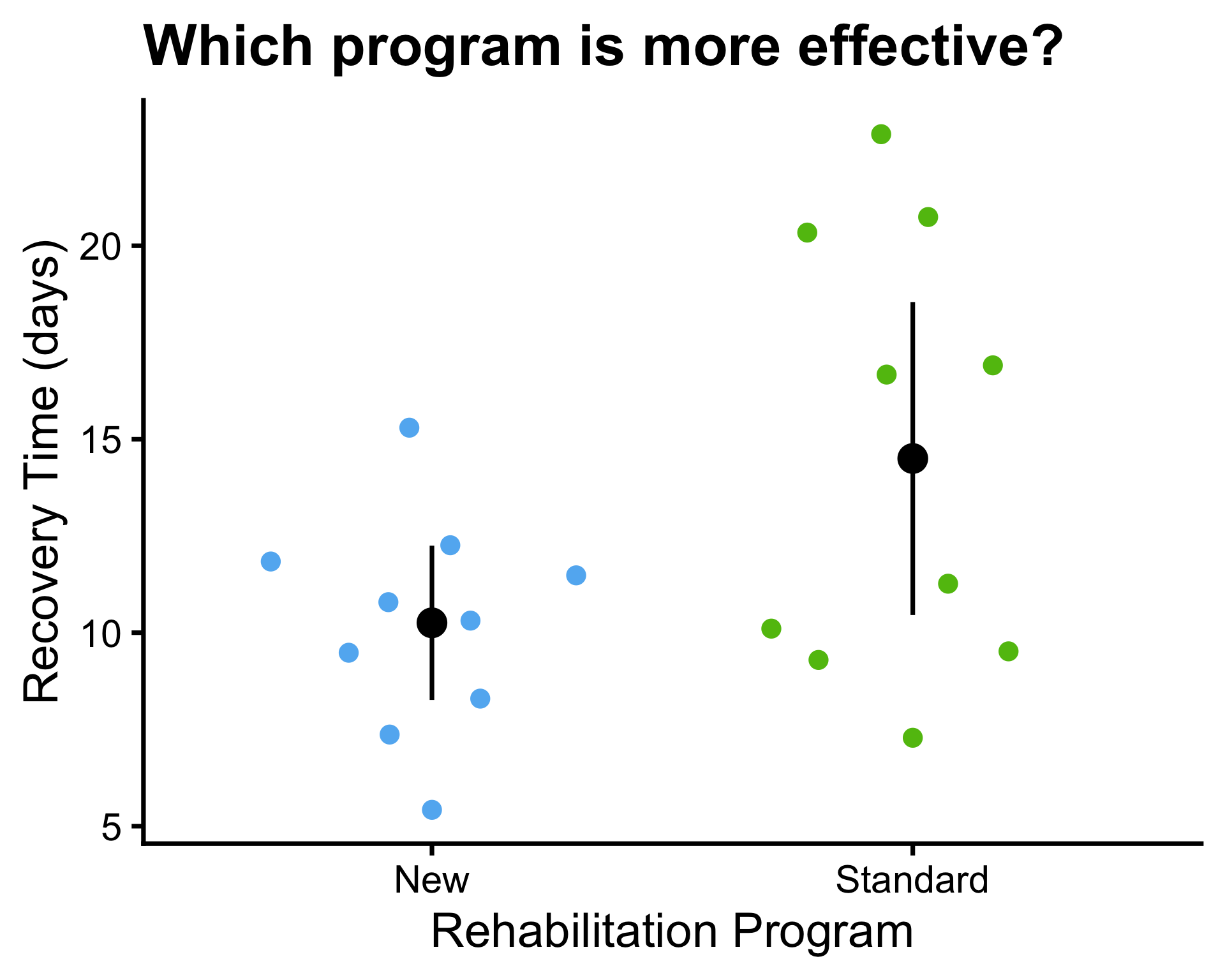
  • \(\mu_1 = 10\) and \(\mu_2 = 14\)
  • \(\bar{x}_1 = 10.3\) and \(\bar{x}_2 = 14.5\)
  • \(\sigma^2_1 = 4\) and \(\sigma^2_2 = 45\)
  • \(s_1^2 = 7.77\) and \(s_2^2 = 31.96\), \(s_p^2 = 19.86\)
  • \(n_1 = 10\) and \(n_2 = 10\)

P-values:

  • Known variance: \(P(Z \leq -1.9) = 0.0287\)
  • Unknown variance: \(P(t_{9} \leq -2.11) = 0.0320\)
  • Unknown equal variances: \(P(t_{18} \leq -2.11) = 0.0246\)
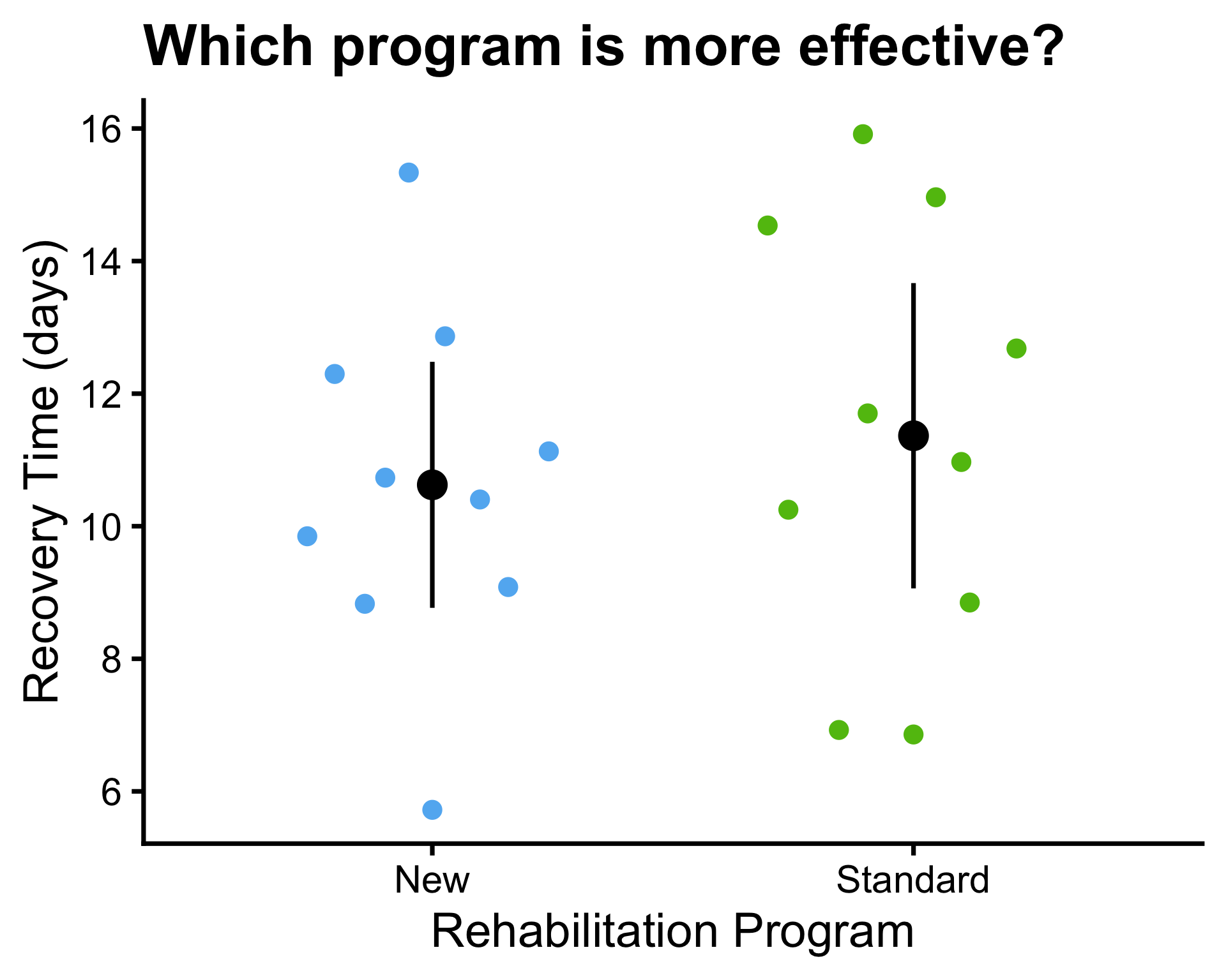
  • \(\mu_1 = 10\) and \(\mu_2 = 10\)
  • \(\bar{x}_1 = 10.6\) and \(\bar{x}_2 = 11.4\)
  • \(\sigma^2_1 = 9\) and \(\sigma^2_2 = 9\)
  • \(s_1^2 = 6.73\) and \(s_2^2 = 10.37\), \(s_p^2 = 8.55\)
  • \(n_1 = 10\) and \(n_2 = 10\)

P-values:

  • Known variance: \(P(Z \leq -0.6) = 0.2743\)
  • Unknown variance: \(P(t_{9} \leq -0.61) = 0.2785\)
  • Unknown equal variances: \(P(t_{18} \leq -0.61) = 0.2747\)
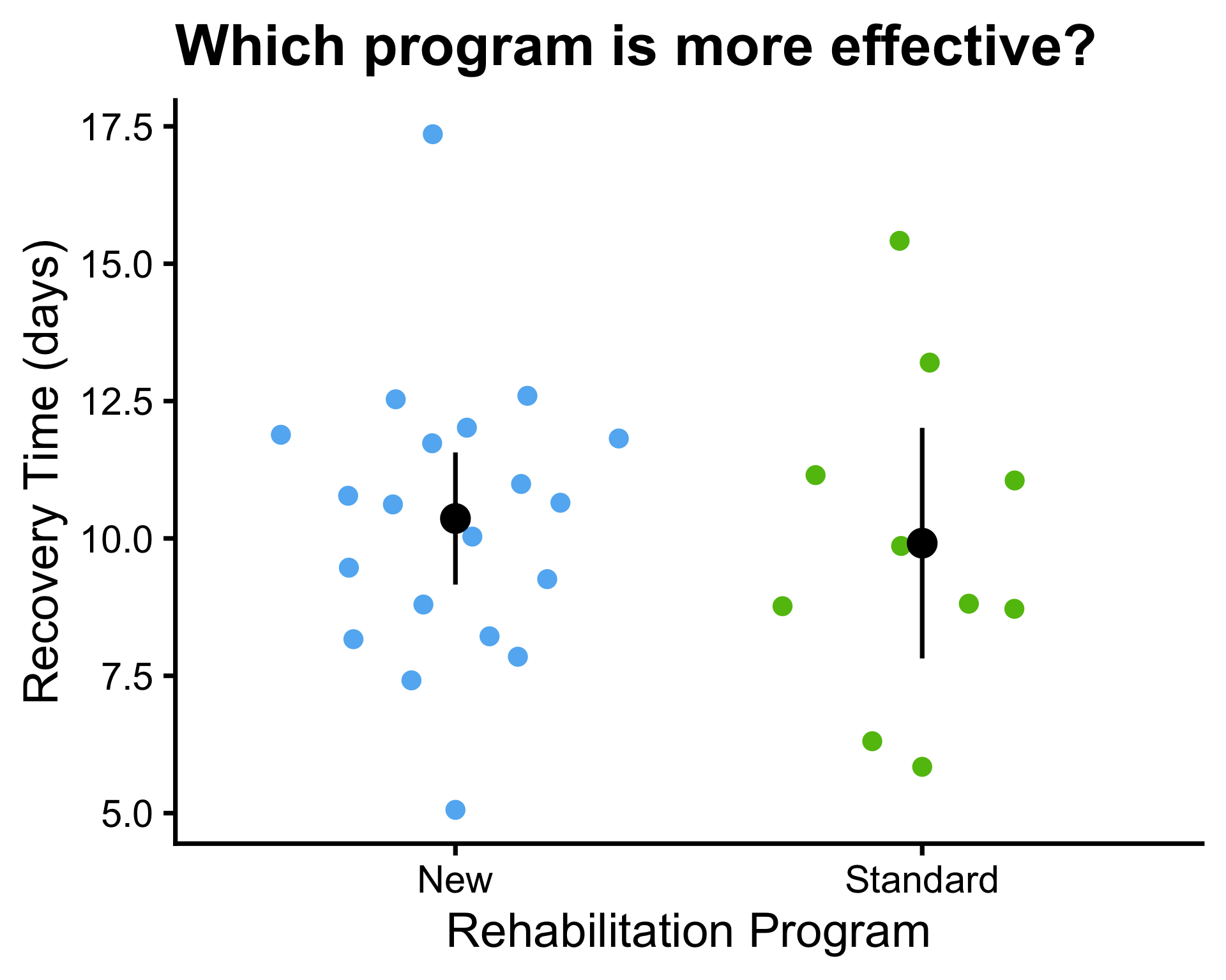
  • \(\mu_1 = 10\) and \(\mu_2 = 10\)
  • \(\bar{x}_1 = 10.4\) and \(\bar{x}_2 = 9.9\)
  • \(\sigma^2_1 = 9.89\) and \(\sigma^2_2 = 10\)
  • \(s_1^2 = 6.61\) and \(s_2^2 = 8.61\), \(s_p^2 = 7.25\)
  • \(n_1 = 20\) and \(n_2 = 10\)

P-values:

  • Known variance: \(P(Z \leq 0.41) = 0.6591\)
  • Unknown variance: \(P(t_{9} \leq 0.46) = 0.6718\)
  • Unknown equal variances: \(P(t_{28} \leq 0.48) = 0.6825\)

Case: Carbon dioxide and growth rate in algae

Growth rates of 14 unicellular alga Chlamydomonas after 1,000 generations of selection under High and Normal levels of carbon dioxide were examined.

Is there a difference in growth rates between the two carbon dioxide levels?

Two sample t-test using R

Assume that:

  • the growth rates are normally distributed, and
  • the samples within and between the two carbon dioxide levels are independent.

Note that:

  • When var.equal = FALSE, the two sample t-test uses the Welch-Satterthwaite approximation for the degrees of freedom (derivation out of scope for this course).
  • When var.equal = TRUE, the two sample t-test assumes that the population variances are equal and uses the pooled variance estimator.

Summary

scroll

\(H_0: \mu_1 = \mu_2\)

  • Observe \(n_1\) samples with sample mean \(\bar{X}_1\) from population 1 with mean \(\mu_1\).
  • Observe \(n_2\) samples with sample mean \(\bar{X}_2\) from population 2 with mean \(\mu_2\).
  • Samples from populations 1 and 2 should be independent.
  • Both populations are normally distributed or sample sizes \(n_1\) and \(n_2\) are sufficiently large.

Test statistic under \(H_0\)

Variances known

\[Z = \dfrac{\bar{X}_{1} - \bar{X}_{2}}{\sqrt{\frac{\sigma_{1}^2}{n_{1}} + \frac{\sigma_{2}^2}{n_{2}}}} \sim N(0, 1)\]

Variances unknown

\[T = \dfrac{\bar{X}_{1} - \bar{X}_{2}}{\sqrt{\frac{s_{1}^2}{n_{1}} + \frac{s_{2}^2}{n_{2}}}} \sim t_{\text{df}}\]

where

  • \(\text{df} = \min(n_{1}, n_{2}) - 1\) if variances cannot not be assumed to be equal and
  • \(\text{df} = n_{1} + n_{2} - 2\) if variances are assumed to be equal and \(s^2_1 = s^2_2 = s^2_p\).
  • \(s_p^2 = \dfrac{(n_{1} - 1)s_{1}^2 + (n_{2} - 1)s_{2}^2}{n_{1} + n_{2} - 2}\) is the pooled variance estimator.

Confidence interval for \(\mu_1 - \mu_2\)

Variances known

\[\bar{X}_{1} - \bar{X}_{2} \pm z_{\alpha / 2} \sqrt{\dfrac{\sigma_{1}^2}{n_{1}} + \dfrac{\sigma_{2}^2}{n_{2}}}\]

Variances unknown

\[\bar{X}_{1} - \bar{X}_{2} \pm t_{\text{df}, \alpha / 2} \sqrt{\dfrac{s_{1}^2}{n_{1}} + \dfrac{s_{2}^2}{n_{2}}}\]

P-value:

Variances known

\(H_A\) P-value
\(H_A: \mu_1 \neq \mu_2\) \(P(|Z| \geq |z^*|)\)
\(H_A: \mu_1 > \mu_2\) \(P(Z \geq z^*)\)
\(H_A: \mu_1 < \mu_2\) \(P(Z \leq z^*)\)

Variances unknown

\(H_A\) P-value
\(H_A: \mu_1 \neq \mu_2\) \(P(|T| \geq |t^*|)\)
\(H_A: \mu_1 > \mu_2\) \(P(T \geq t^*)\)
\(H_A: \mu_1 < \mu_2\) \(P(T \leq t^*)\)