Acknowledgement

This lecture was partially adapted from the previous STAT1003 lecturers. Thank you folks!

Hypothesis Testing

Statistical inference

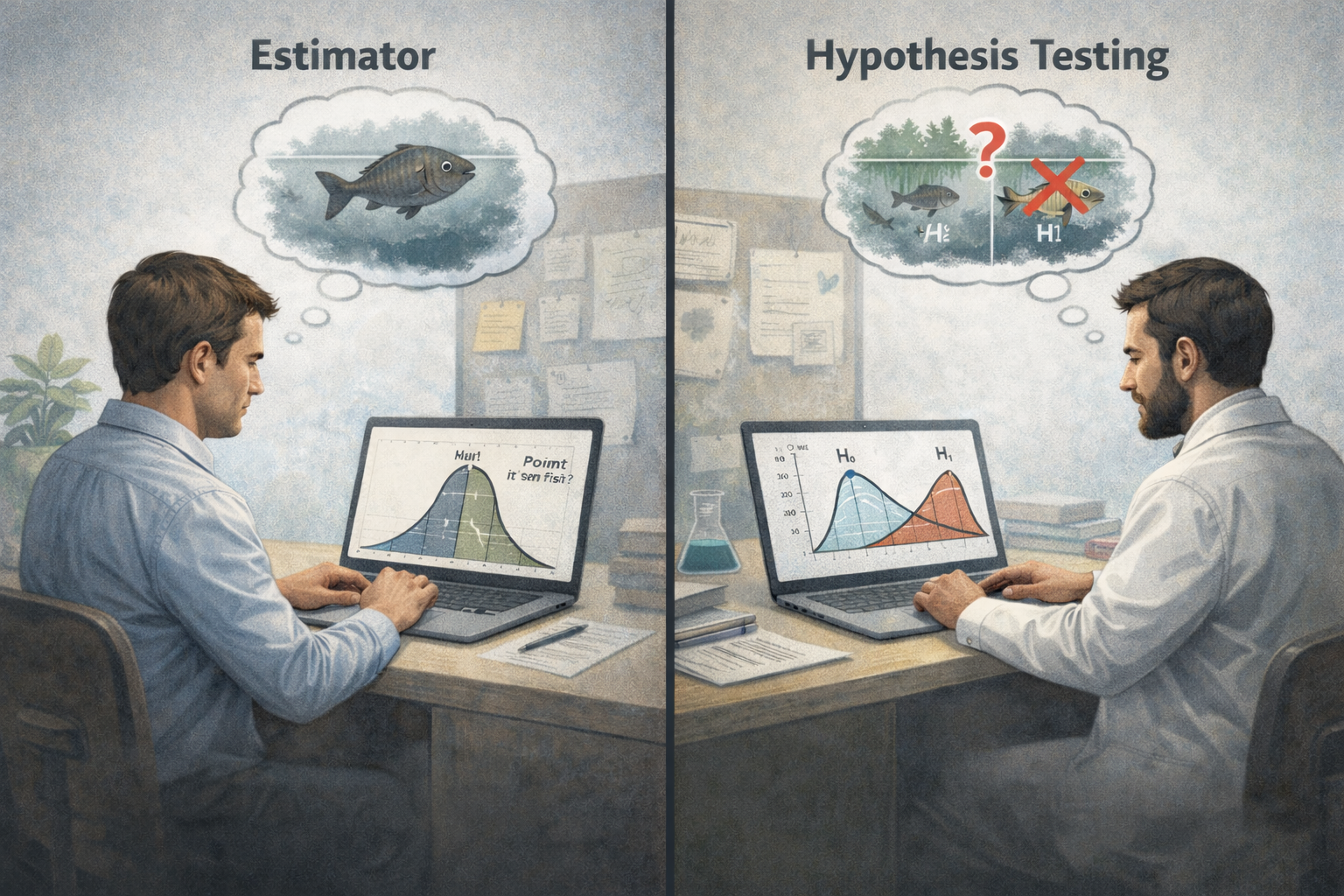
Estimation (last topic)

Draw inferences about a population by estimating population parameters from a sample (point and interval estimators).

Hypothesis testing (this topic)

Draw inferences about a population by making a claim or hypothesis about a population parameter and testing whether the hypothesis is supported by the sample.
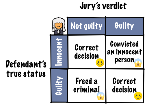


The judicial system

  • In a criminal court case, the defendant is either:
    1. guilty of the alleged crime or
    2. not guilty of the alleged crime.
  • The prosecutor and the defence lawyer present their evidence with assumptions to the jury and/or judge during the trial.
  • The jury has to decide whether to convict the defendant or not based on the evidence.

The “statistical” judicial system

  • In a “statistical” court case, there are two competing hypotheses:
    1. The null hypothesis (\(H_0\)) or
    2. The alternative hypothesis (\(H_A\) or \(H_1\)).
  • A sample of data is collected and a test statistic under assumptions provides evidence to test the \(H_0\).
  • Based on the strength of evidence, we decide whether to reject the \(H_0\) or not.

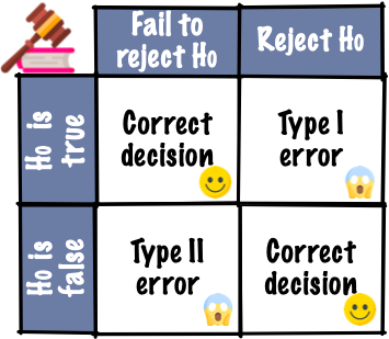
Two types of errors can occur in this process:

  1. Type I error: rejecting the \(H_0\) when it is actually true.
  2. Type II error: failing to reject the \(H_0\) when the \(H_A\) is actually true.

Null hypothesis \(H_0\) and alternative hypothesis \(H_A\)

  • The null hypothesis, denoted as \(H_0\), is a statement about a population parameter (e.g. \(\theta = \theta_0\)) that we want to test.
  • \(H_0\) often represents a “status quo” or “no effect” scenario.
  • \(H_0\) is assumed to be true until evidence suggests otherwise.
  • The alternative hypothesis, denoted as \(H_A\) (or \(H_1\)), is a contrary statement to \(H_0\) that we want to provide evidence for.
  • The alternative hypothesis can be:
    • two-sided: \(H_A: \theta \neq \theta_0\) (two-tail test), or
    • one-sided: \(H_A: \theta > \theta_0\) (upper-tail test) or \(H_A: \theta < \theta_0\) (lower-tail test).

State the hypotheses

Determine the null and alternative hypotheses based on the research question.

The packaging on a light bulb states that the bulb will last 500 hours under normal use. A consumer advocate would like to know if the mean lifetime of a bulb is less than 500 hours.

According to an Australian Bureau of Statistics survey conducted in 2010, 77% of Australian adults were mostly or extremely satisfied with their life as a whole. A researcher wonders if the percentage of satisfied Australians is the same today.

A sports dietician would like to see whether the intake of caffeine prior to a race can improve the performance of ultra marathon runners.

Hypothesis Testing for Population Proportion

Example: Is this coin biased towards heads?

  • Suppose I have a coin that I’m going to flip

  • I have some suspicion that the coin has been tweaked to be biased towards heads.

  • Let \(p\) be the probability of getting a head.

  • If the coin is biased towards heads, then

  • So how would we test if a coin is biased towards head or not?

  • We’ll collect some data.

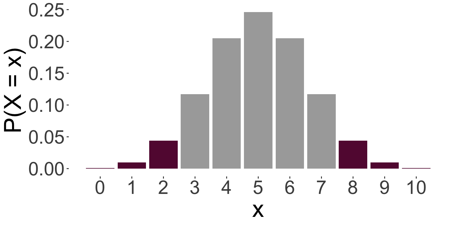
I flipped the coin 10 times and this is the result:

  • The result is 7 head and 3 tails. So 70% are heads.
  • Do you believe the coin is biased towards heads based on this data?

Example: Is this coin biased towards heads?

Suppose now I flip the coin 200 times and this is the outcome:

  • We observe 140 heads and 60 tails. So again 70% are heads.
  • Based on this data, do you think the coin is biased towards heads?
  • If the coin was fair, how many heads did you expect to see?

A one-sided binomial test

  • Suppose \(X\) is the number of heads out of \(n\) independent tosses.
  • Let \(p\) be the probability of getting a head for this coin.
  • Hypotheses: \(H_0: p = 0.5\) vs. \(H_A: p > 0.5\)
  • Assumptions: Each toss is independent with equal chance of getting a head.
  • Test statistic: \(X \sim B(n, p)\) under \(H_0\).
    • Let \(x\) be the observed number of heads.
    • High value of \(x\) suggests that the coin is biased towards heads (\(p > 0.5\)).
  • P-value: The probability of observing a test statistic as extreme or more extreme than the one observed, assuming \(H_0\) is true. For \(H_A: p > 0.5\), p-value \(= P(X \geq x)\).
  • Conclusion: Select a significance level \(\alpha\) (e.g. \(\alpha = 0.05\)).
    • If p-value < \(\alpha\), the observed data is unlikely to have occurred under \(H_0\).
    • If p-value \(\geq \alpha\), the observed data is consistent with \(H_0\).

Example: calculating the p-value for \(H_A: p > 0.5\)

\(H_0: p = 0.5\) vs. \(H_A: p > 0.5\)

We observed \(x = 7\) heads out of \(n = 10\) tosses.

The p-value is \(P(X \geq x) = 1 - P(X \leq x - 1) = 1 - P(X \leq 6)\).

We observed \(x = 140\) heads out of \(n = 200\) tosses.

The p-value is \(P(X \geq x) = 1 - P(X \leq x - 1) = 1 - P(X \leq 139)\).

Significance level \(\alpha\) and Type I error

  • The significance level \(\alpha\) is the threshold for rejecting the null hypothesis.
  • It is the probability of making a Type I error: rejecting the null hypothesis when it is actually true.
  • Common choices for \(\alpha\) are 0.05, 0.01, or 0.10, but the choice should depend on the context of the problem and the consequences of making a Type I error.
  • If the data is generated under \(H_0\), the p-value follows roughly a uniform distribution on [0, 1].

A two-sided binomial test

  • Hypothesis tests can also be two-sided.
  • Hypothesis: \(H_0: p = 0.5\) vs. \(H_A: p \neq 0.5\)
  • Assumptions: Each toss is independent with equal chance of getting a head.
  • Test statistic: \(X \sim B(n, p)\) under \(H_0\).
    • Let \(x\) be the observed number of heads.
    • High or low values of \(x\) suggests that the coin is biased.

  • P-value: the probability of observing a test statistic as extreme or more extreme than the one observed, assuming \(H_0\) is true. For a two-sided test, this is \[P(|X - E(X)| \geq |x - E(X)|).\]
  • Conclusion: Select a false positive rate \(\alpha\) (e.g. \(\alpha = 0.05\)).
    • If p-value < \(\alpha\), the observed data is unlikely to have occurred under \(H_0\).
    • If p-value \(\geq \alpha\), the observed data is consistent with \(H_0\).

Example: calculating the p-value for \(H_A: p \neq 0.5\)

\(H_0: p = 0.5\) vs. \(H_A: p \neq 0.5\)

We observed \(x = 7\) heads out of \(n = 10\) tosses.

The p-value is \(P(|X - E(X)| \geq |x - E(X)|) = P(|X - 5| \geq 2) = P(X \leq 3) + P(X \geq 7)\).

We observed \(x = 140\) heads out of \(n = 200\) tosses.

The p-value is \(P(|X - 100| \geq 40) = P(X \leq 60) + P(X \geq 140)\).

Binomial test (two-sided) with R

\(H_0: p = 0.5\) vs. \(H_A: p \neq 0.5\)

Binomial test (one-sided) with R

Note: if performing a one-sided test, the directon should have been specified in advance of the experiment.


Upper-tail test: \(H_0: p = 0.5\) vs. \(H_A: p > 0.5\)

Lower-tail test: \(H_0: p = 0.5\) vs. \(H_A: p < 0.5\)

Null hypothesis significance testing: Conclusion

  • Conclusion: Reject \(H_0\) when the p-value is less than some significance level \(\alpha\).
  • Usually \(\alpha = 0.05\), but some argue it should be even lower.
  • There has been a lot of misuse of p-values in scientific research that American Statistical Association (ASA) issued a statement on p-values.

The ASA statement on p-values highlights the following six principles:

  1. P-values can indicate how incompatible the data are with a specified statistical model.
  2. P-values do not measure the probability that the studied hypothesis is true, or the probability that the data were produced by random chance alone.
  3. Scientific conclusions and business or policy decisions should not be based only on whether a p-value passes a specific threshold.
  4. Proper inference requires full reporting and transparency.
  5. A p-value, or statistical significance, does not measure the size of an effect or the importance of a result.
  6. By itself, a p-value does not provide a good measure of evidence regarding a model or hypothesis.

Confidence interval for hypothesis testing

In light of misuses of and misconceptions concerning p-values, the statement notes that statisticians often supplement or even replace p-values with other approaches. These include methods “that emphasize estimation over testing such as confidence … intervals”

— ASA Statement on p-values

If \(H_0: p = p_0\) vs \(H_A: p \neq p_0\) and the \(100(1-\alpha)\)% confidence interval contains \(p_0\), then we fail to reject the null hypothesis at \(\alpha\) significance level.

  • Here the 95% confidence interval does not contain \(p_0 = 0.5\), therefore the null hypothesis is rejected at \(\alpha = 0.05\) significance level.

Summary

Hypothesis testing is a systematic way to evaluate evidence against a null hypothesis. It involves:

  • Hypothesis: Formulating null \(H_0\) and alternative \(H_A\) hypotheses.
  • Assumptions: Specifying assumptions about the data and the test statistic.
  • Test statistic: Choosing an appropriate test statistic based on the hypotheses and assumptions.
  • P-value: The probability of observing a test statistic as extreme or more extreme than the one observed, assuming the null hypothesis is true.
  • Conclusion: Making a decision to reject (p-value \(< \alpha\)) or fail to reject (p-value \(\geq \alpha\)) the null hypothesis based on the p-value and a predetermined significance level \(\alpha\).

Binomial test \(H_0: p = p_0\)

  • Test statistic: \(X \sim B(n, p_0)\) under \(H_0\).
  • P-value:
    • \(H_A: p > p_0\) (upper-tail test) \(\rightarrow\) p-value = \(P(X \geq x)\)
    • \(H_A: p < p_0\) (lower-tail test) \(\rightarrow\) p-value = \(P(X \leq x)\)
    • \(H_A: p \neq p_0\) (two-tail test) \(\rightarrow\) p-value = \(P(|X - np_0| \geq |x - np_0|)\)

Hypothesis Testing for Population Mean

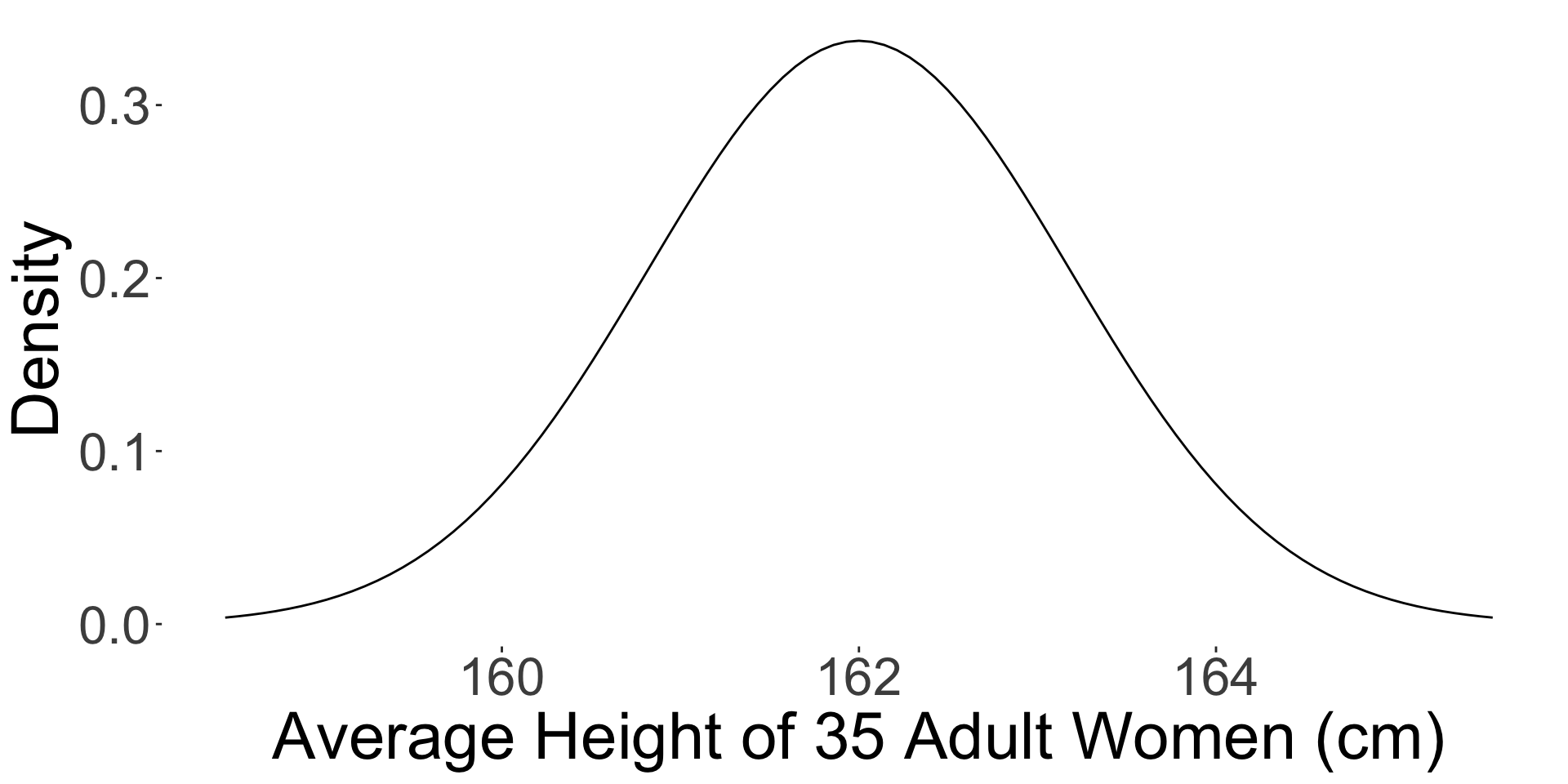
Example: adult height

I am 160 cm tall.

Am I significantly shorter than the average adult woman in Australia?

  • I collect a random sample of 35 adult women in Australia and measure their heights.
  • The sample mean height is 162 cm and the sample standard deviation is 7 cm.
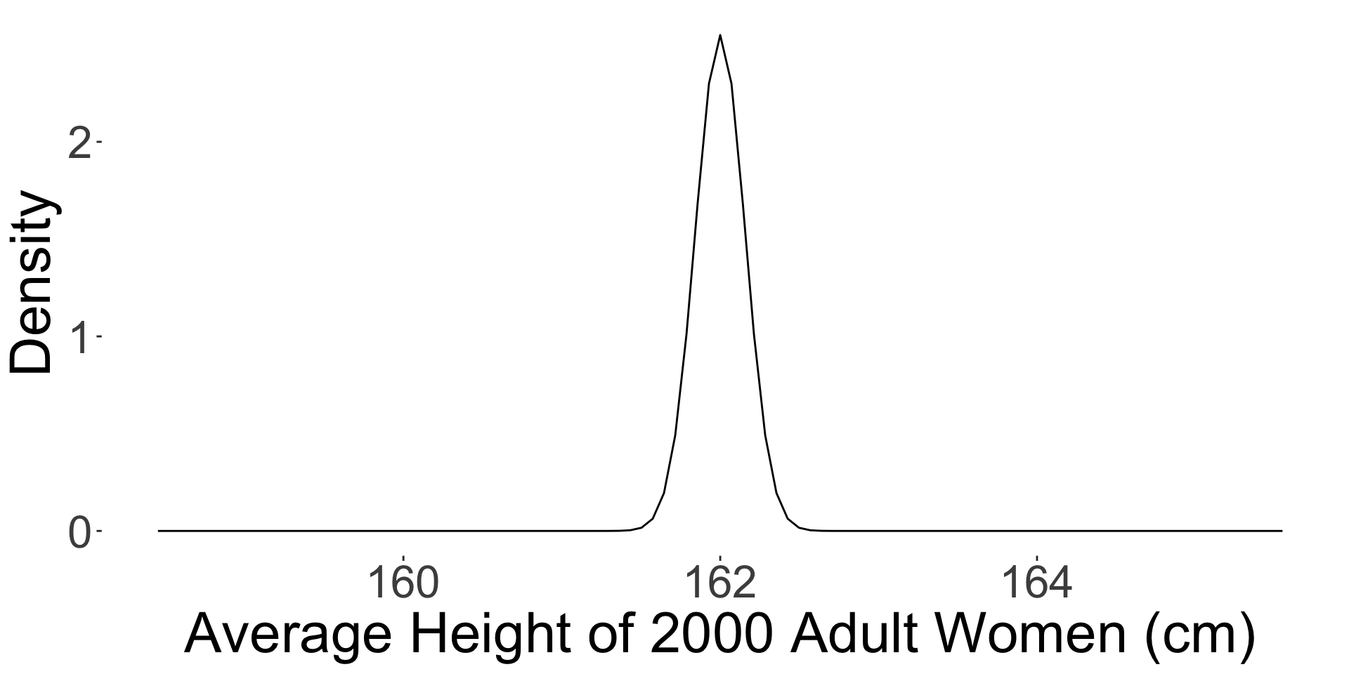
  • I collect a random sample of 2000 adult women in Australia and measure their heights.
  • The sample mean height is 162 cm and the sample standard deviation is 7 cm.


Testing for the population mean

\(H_0: \mu = \mu_0\) vs. \(H_A: \mu \neq \mu_0\) or \(H_A: \mu > \mu_0\) or \(H_A: \mu < \mu_0\)

We observe \(n\) samples from a population with mean \(\mu\) and standard deviation \(\sigma\).

  • The test statistic for population mean is often the sample mean \(\bar{X}\) or its standardized form:
    • \(Z = \dfrac{\bar{X} - \mu_0}{\sigma / \sqrt{n}}\) if \(\sigma\) is known, or
    • \(T = \dfrac{\bar{X} - \mu_0}{S / \sqrt{n}}\) if \(\sigma\) is unknown, where \(S\) is the sample standard deviation.
  • For large \(n\) or if the population is normally distributed:
    • \(Z \sim N(0, 1)\) under \(H_0\), and
    • \(T \sim t_{n-1}\) under \(H_0\).

Decisions in hypothesis testing

  • We have so far used the p-value to make a conclusion in hypothesis testing.
  • For \(H_0: \mu = \mu_0\) vs.
    • \(H_A: \mu > \mu_0\), p-value = \(P(Z \geq z^*)\) or \(P(T \geq t^*)\),
    • \(H_A: \mu < \mu_0\), p-value = \(P(Z \leq z^*)\) or \(P(T \leq t^*)\),
    • \(H_A: \mu \neq \mu_0\), p-value = \(P(|Z| \geq |z^*|)\) or \(P(|T| \geq |t^*|)\).
  • We reject \(H_0\) if p-value < \(\alpha\) and fail to reject \(H_0\) if p-value \(\geq \alpha\).
  • Or for a two-sided test, we can:
    • reject \(H_0\) if the confidence interval does not contain \(\mu_0\) and
    • data is consistent with \(H_0\) or fail to reject \(H_0\) if the confidence interval contains \(\mu_0\).
  • Or we check if the test statistic falls in the rejection region (reject \(H_0\)) or not (fail to reject \(H_0\)).
  • Note: we say “fail to reject \(H_0\)” instead of “accept \(H_0\) because we can never be sure that \(H_0\) is true. We can alternatively say that the data is consistent with \(H_0\).

Rejection region for hypothesis testing

The rejection region is the set of values of the test statistic that leads to rejection of \(H_0\).

  • For \(H_0: \mu = \mu_0\):
Alternative Hypothesis Rejection Region for \(\sigma\) known Rejection Region for \(\sigma\) unknown
\(H_A: \mu > \mu_0\) \((z^*_{\alpha}, \infty)\) \((t^*_{n - 1, \alpha}, \infty)\)
\(H_A: \mu < \mu_0\) \((-\infty, z^*_{\alpha})\) \((-\infty, t^*_{n - 1, \alpha})\)
\(H_A: \mu \neq \mu_0\) \((-|z^*_{\alpha/2}|, |z^*_{\alpha/2}|)\) \((-|t^*_{n - 1, \alpha/2}|, |t^*_{n - 1, \alpha/2}|)\)


where the critical values are defined as:

  • \(z^*_{\alpha}\) is such that \(P(Z \geq z^*_{\alpha}) = \alpha\) for \(Z \sim N(0, 1)\), and
  • \(t^*_{n - 1, \alpha}\) is such that \(P(T \geq t^*_{n - 1, \alpha}) = \alpha\) for \(T \sim t_{n - 1}\).

Example: calculating the p-value

I am 160 cm tall. Am I significantly shorter than the average adult woman in Australia?

\(H_0: \mu = 160\) (I’m average height) vs. \(H_A: \mu > 160\) (I am shorter than the population average)

One-sample t-test with R

Statistical vs. Practical significance

\(H_0: \mu_1 = \mu_2\) vs. \(H_A: \mu_1 \neq \mu_2\)

  • The above code generates two samples of one million observations each from normal distributions with means 0 and 0.0001, respectively, and standard deviation 0.01.
  • The true difference in means is 0.0001, but the p-value will be much less than 0.05 in most cases.
  • While the difference is statistically significant, it may not be practically significant.
  • So look at the actual difference or “effect size” in addition to the context of the data.

Type II Error and Power

  • Recall Type II Error is failing to reject \(H_0\) when \(H_A\) is actually true.
  • Let \(\beta = P(\text{Type II error})\) be the probability of making a Type II error.

The power of a test is defined as \(1 - \beta\), which is the probability of correctly rejecting \(H_0\) when \(H_A\) is true.

  • The true parameter value under \(H_A\) is often unknown, so we cannot calculate \(\beta\) or power directly from the data.
  • However, we can calculate \(\beta\) or power for a specific parameter value under \(H_A\) using the distribution of the test statistic under that parameter value.
  • Power calculations are often used in the design phase of a study to determine the required sample size to achieve a desired level of power for detecting a meaningful effect size.

Calculating Type II Error

The population adult woman mean height is 165 cm and population standard deviation is 15 cm. What is the probability that we will make a Type II Error if we collect a new sample of size 35 and conduct hypothesis testing with significance level 0.05?

  • \(H_0: \mu = 160\) vs. \(H_A: \mu > 160\)
  • The critical value for \(\alpha = 0.05\) is \(z^*_{0.05} = 1.645\), so we fail to reject \(H_0\) if \[Z = \dfrac{\bar{X} - 160}{15 / \sqrt{35}}< 1.645 \rightarrow \bar{X} < 160 + 1.645 \times \frac{15}{\sqrt{35}} = 164.1708.\]
  • \(P(\text{Type II error}) = P(\bar{X} < 164.1708 \mid \mu = 165)\), i.e. \(\bar{X} \sim N(165, 15^2 / 35)\) under \(H_A: \mu = 165\).

Summary

Hypothesis testing for a single population mean:

  1. Hypotheses: State the null and alternative hypotheses.
  2. Assumptions: Check the assumptions or conditions for the test.
  3. Test Statistic: Calculate the observed test statistic \(\bar{x}\) or its standardized form \(z^* = \frac{\bar{x} - \mu_0}{\sigma / \sqrt{n}}\) (\(\sigma\) is known) or \(t^* = \frac{\bar{x} - \mu_0}{s / \sqrt{n}}\) (\(\sigma\) is unknown) and \(Z\sim N(0, 1)\) or \(T \sim t_{n-1}\) under \(H_0\).
  4. P-value or confidence Interval or rejection region: \(H_0: \mu = \mu_0\):
\(H_A\) P-value Confidence Interval Rejection Region
\(\mu > \mu_0\) \(P(Z \geq z^*)\) or \(P(T \geq t^*)\) - \((z^*_{\alpha}, \infty)\) or \((t^*_{n - 1, \alpha}, \infty)\)
\(\mu < \mu_0\) \(P(Z \leq z^*)\) or \(P(T \leq t^*)\) - \((-\infty, z^*_{\alpha})\) or \((-\infty, t^*_{n - 1, \alpha})\)
\(\mu \neq \mu_0\) \(P(|Z| \geq |z^*|)\) or \(P(|T| \geq |t^*|)\) \(\bar{x} \pm z^*_{\alpha/2} \frac{\sigma}{\sqrt{n}}\) or \(\bar{x} \pm t^*_{n-1, \alpha/2} \frac{s}{\sqrt{n}}\) \((-|z^*_{\alpha/2}|, |z^*_{\alpha/2}|)\) or \((-|t^*_{n - 1, \alpha/2}|, |t^*_{n - 1, \alpha/2}|)\)
  1. Conclusion: For a given significance level \(\alpha\), draw conclusion based on whether:
  • p-value \(< \alpha\) or not, or
  • confidence interval contains \(\mu_0\) or not for a two-sided test only, or
  • observed test statistic falls in the rejection region or not.

Always interpret the results of hypothesis testing in the context of the data and the research question.