Interval estimators
STAT1003 – Statistical Techniques
Australian National University
These slides are best viewed on a modern browser like Google Chrome on a desktop or laptop. Some interactive components may require some time to fully load.
Interval estimators
- Point estimators will almost always be wrong.
- Instead of giving a single value, we can give a range of plausible values for the parameter.
- This range is called an interval estimator.
- We will focus on a specific type of interval estimator called a confidence interval.

A \(100(1 - \alpha)\%\) confidence interval for \(\mu\) when \(\sigma\) is known
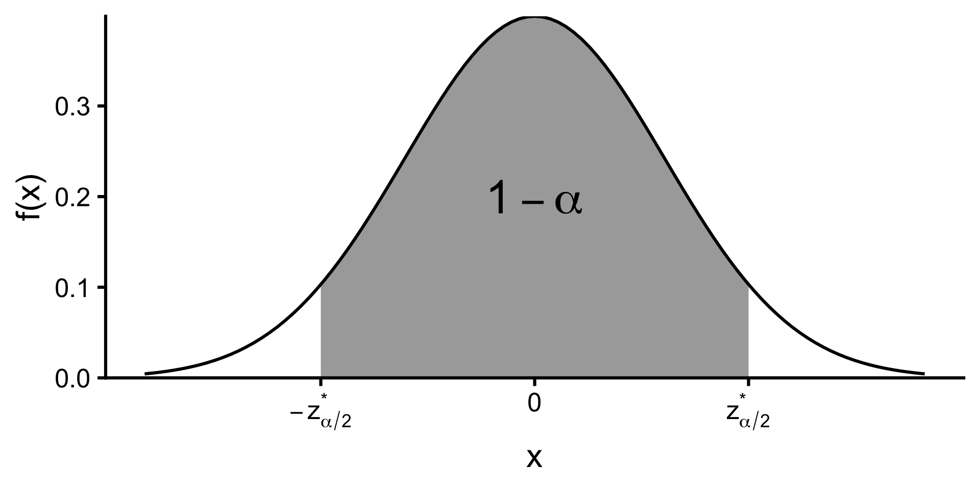
\[\left(\bar{X}-z^*_{\alpha/2}\frac{\sigma}{\sqrt{n}},\;\bar{X}+z^*_{\alpha/2}\frac{\sigma}{\sqrt{n}}\right)\]
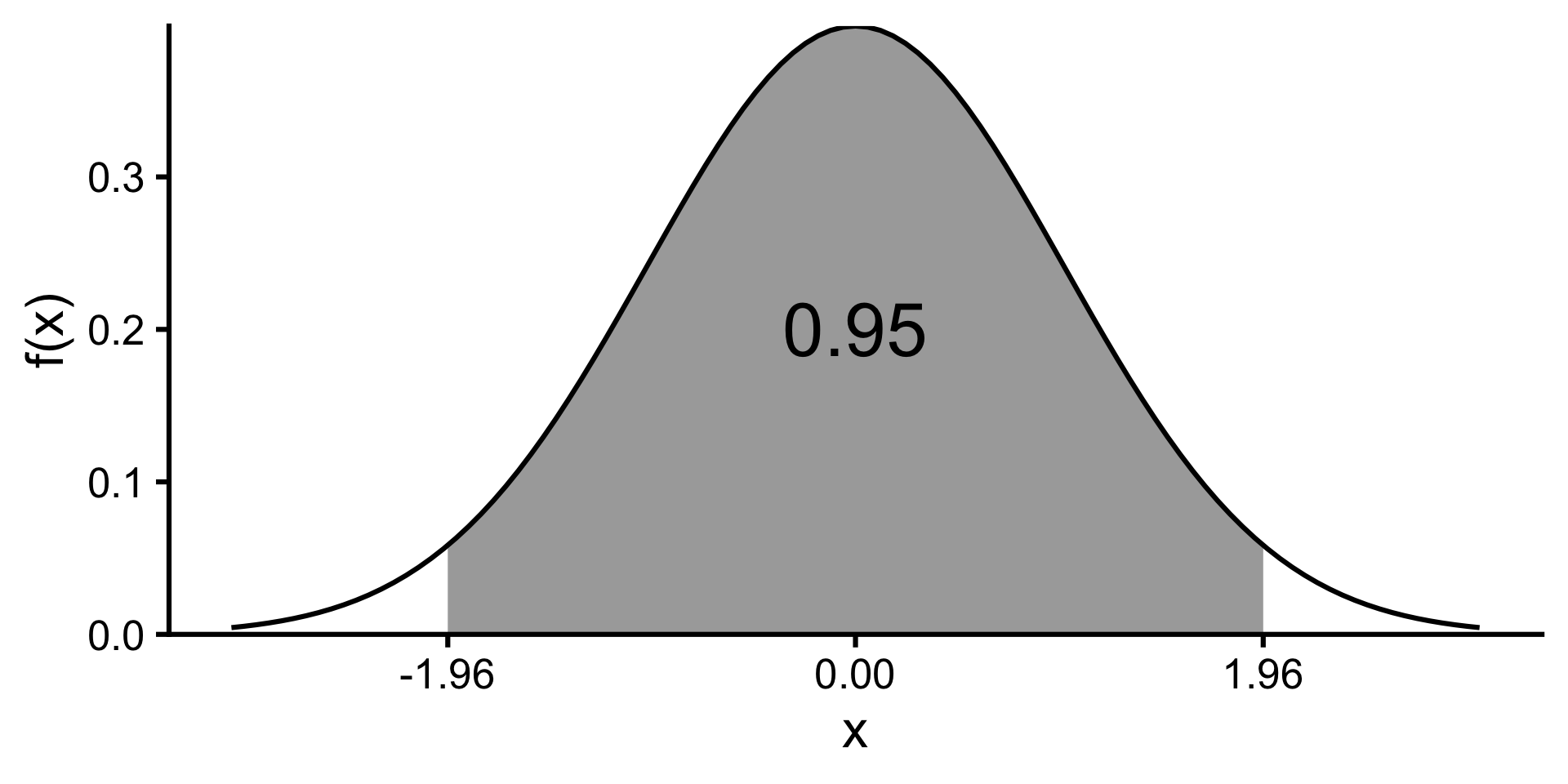
where \(z^*_{\alpha/2}\) is the critical value such that \[P(Z < z^*_{\alpha/2}) = 1 - \alpha/2\] for \(Z \sim N(0,1)\).
Factors affecting the width of a confidence interval
- Sample size: Larger \(n\) → narrower interval.
- Confidence level: Higher confidence → wider interval.
- Population variability: More variability → wider interval.
\[\left(\bar{X}-z^*_{\alpha/2}\frac{\sigma}{\sqrt{n}},\;\bar{X}+z^*_{\alpha/2}\frac{\sigma}{\sqrt{n}}\right)\]
