Point and Interval Estimators

STAT1003 – Statistical Techniques

Dr. Emi Tanaka

Australian National University

These slides are best viewed on a modern browser like Google Chrome on a desktop or laptop. Some interactive components may require some time to fully load.

Acknowledgement

This lecture was partially adapted from the previous STAT1003 lecturers. Thank you folks!

Point Estimators

Point estimator

We use statistics as estimators for the population parameters.

Estimator: the formula or method, e.g., \(\bar{X}\) as estimator for \(\mu\).
Estimate: the number you get when you apply the method to data, e.g. \(\bar{x} = 63.2\).

Let \(\theta\) be some population parameter and let \(\hat{\theta}\) denote a point estimator of \(\theta\).

Case study: a point estimator for \(\mu\)

Why should we use the sample mean \(\bar{X}\) as a point estimator for the population mean \(\mu\)?

Consider three different point estimators for \(\mu\):

The sample mean: \(\hat{\theta}_1 = \bar{X}\) (the sample mean)
The sample median: \(\hat{\theta}_2 = \tilde{X}\) (the sample median)
The average of the first two observations: \(\hat{\theta}_3 = \dfrac{1}{2}(X_1 + X_2)\)

Which estimator is “better”?

The error of a point estimate

In practice, the estimated value is almost never exactly equal to the unknown population parameter value.

Error of the estimate is the difference between the estimated value and the parameter, and is composed of:

Bias describes a systematic tendency to over- or under-estimate the true population value
Sampling error describes the variability of the estimator from one sample to another \[\underbrace{\hat{\theta}- \theta}_{\large \text{Error}} = \underbrace{\hat{\theta} - \text{E}(\hat{\theta})}_{\large \text{Sampling Error}} + \underbrace{\text{E}(\hat{\theta}) - \theta}_{\large \text{Bias}}\]

We evaluate a point estimator in these two aspects.

Bias of a point estimator

Bias of a point estimator describes its systematic tendency to over- or under-estimate the true population value.

The formal definition of the bias of a point estimator \(\hat{\theta}\) of a parameter \(\theta\) is

\[\text{Bias}(\hat{\theta}) = E(\hat{\theta}) - \theta\]

A point estimator is unbiased if \(\text{Bias}(\hat{\theta}) = 0\), i.e. if \(\text{E}(\hat{\theta}) = \theta\)
- If the bias is positive, the estimator tends to over-estimate the parameter.
- If the bias is negative, the estimator tends to under-estimate the parameter.

Case study: bias of a point estimator

We have shown before that \(E(\bar{X}) = \mu\), so sample mean \(\bar{X}\) is an unbiased estimator for \(\mu\).

The sample median, \(\tilde{X}\), would:

be an unbiased estimator only if the population distribution is symmetric,
have a positive bias if the population distribution is right-skewed, and
have a negative bias if the population distribution is left-skewed.

If we use the average of the first two observations in the sample as an estimator, this would also be an unbiased estimator because

\[ E\left[\frac{1}{2}(X_{1} + X_{2})\right] = \frac{1}{2}\left[E(X_{1}) + E(X_{2})\right] = \frac{1}{2}(\mu + \mu) = \mu. \]

Variance of a point estimator

Sampling error, sometimes called sampling uncertainty, describes how much an estimate will tend to vary from one sample to the next.
It is measured by the variance of an estimator.
If \(\hat{\theta}\) is a point estimator of \(\theta\), the variance of \(\hat{\theta}\) is

\[\text{Var}(\hat{\theta}) = E\left((\hat{\theta} - E(\hat{\theta}))^2\right) = E\left(\hat{\theta}^2\right) - \left(E(\hat{\theta})\right)^2\]

Estimators with low variance are said to be efficient, i.e. for two unbiased estimators \(\hat{\theta}_1\) and \(\hat{\theta}_2\), if \(\text{Var}(\hat{\theta}_1) < \text{Var}(\hat{\theta}_2)\) then \(\hat{\theta}_1\) is considered more efficient.

Case study: variance of a point estimator

\(\text{Var}(\bar{X}) = \dfrac{\sigma^2}{n}\)

The variance decreases when the sample size increases.
We will get a more efficient estimator for the population mean when the sample size is large.

\(\text{Var}(\tilde{X}) \approx \dfrac{\pi\sigma^2}{2n}\) if the population distribution is normal (proof out of scope).

It is less efficient than the sample mean.

\(\text{Var}\left[\frac{1}{2}(X_1 + X_2)\right] = \frac{1}{4}\left[\text{Var}(X_1) + \text{Var}(X_2)\right] = \frac{1}{4}\left[\sigma^2 + \sigma^2\right] = \dfrac{\sigma^2}{2}\)

It is less efficient than the sample mean when \(n > 2\).

Case study: variance of a point estimator via simulation

Mean squared error of a point estimator

To evaluate a point estimator, we need to consider both its bias and its variance.

The mean squared error (MSE) of a point estimator takes into account both. It is defined as

\[\text{MSE}(\hat{\theta}) = \text{E}\left[(\hat{\theta} - \theta)^2\right] = \left(\text{E}(\hat{\theta}) - \theta\right)^2 + E\left((\hat{\theta} - E(\hat{\theta}))^2\right) = \text{Bias}(\hat{\theta})^2 + \text{Var}(\hat{\theta})\]

MSE is often used as a criterion for comparing estimators.

Consistency of a point estimator

A point estimator is said to be consistent if the MSE of the estimator goes to zero as sample size \(n\) increases:

\[\lim_{n \to \infty} \text{MSE}(\hat{\theta}) = 0\]

Summary

Unbiasedness: The estimator’s expected value equals the true parameter: \(\text{E}(\hat{\theta}) = \theta\).
Efficiency: Among unbiased estimators, the one with the smallest variance is preferred: \(\text{Var}(\hat{\theta}) < \text{Var}(\hat{\theta}')\)
Consistency: As sample size increases, the estimator gets closer to the true parameter: \(\lim_{n \to \infty} \text{MSE}(\hat{\theta}) = 0\).

Interval Estimators

Interval estimators

Point estimators will almost always be wrong.
Instead of giving a single value, we can give a range of plausible values for the parameter.
This range is called an interval estimator.
We will focus on a specific type of interval estimator called a confidence interval.

Confidence intervals for a population mean

A 95% confidence interval for \(\mu\) when \(\sigma\) is known

Use the sample mean \(\bar{X}\) as the point estimator for \(\mu\).
By the CLT, \(\bar{X} \overset{\text{approx}}{\sim} N\!\left(\mu, \dfrac{\sigma^2}{n}\right)\) for large \(n\).

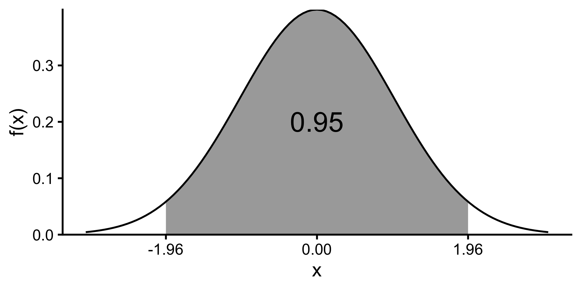
For a standard normal variable, \(P(-1.96 < Z < 1.96) \approx 0.95\).

\[\begin{align*} & P\left(-1.96 < \frac{\bar{X} - \mu}{\sigma/\sqrt{n}} < 1.96\right) \approx 0.95\\ &\quad = P\left(-1.96\frac{\sigma}{\sqrt{n}} < \bar{X} - \mu < 1.96\frac{\sigma}{\sqrt{n}}\right) \\ &\quad = P\left(\bar{X}-1.96\frac{\sigma}{\sqrt{n}} < \mu < \bar{X}+1.96\frac{\sigma}{\sqrt{n}}\right) \\ \end{align*}\]

Therefore, a 95% confidence interval for \(\mu\) is \[\left(\bar{X}-1.96\frac{\sigma}{\sqrt{n}},\;\bar{X}+1.96\frac{\sigma}{\sqrt{n}}\right).\]

A \(100(1 - \alpha)\%\) confidence interval for \(\mu\) when \(\sigma\) is known

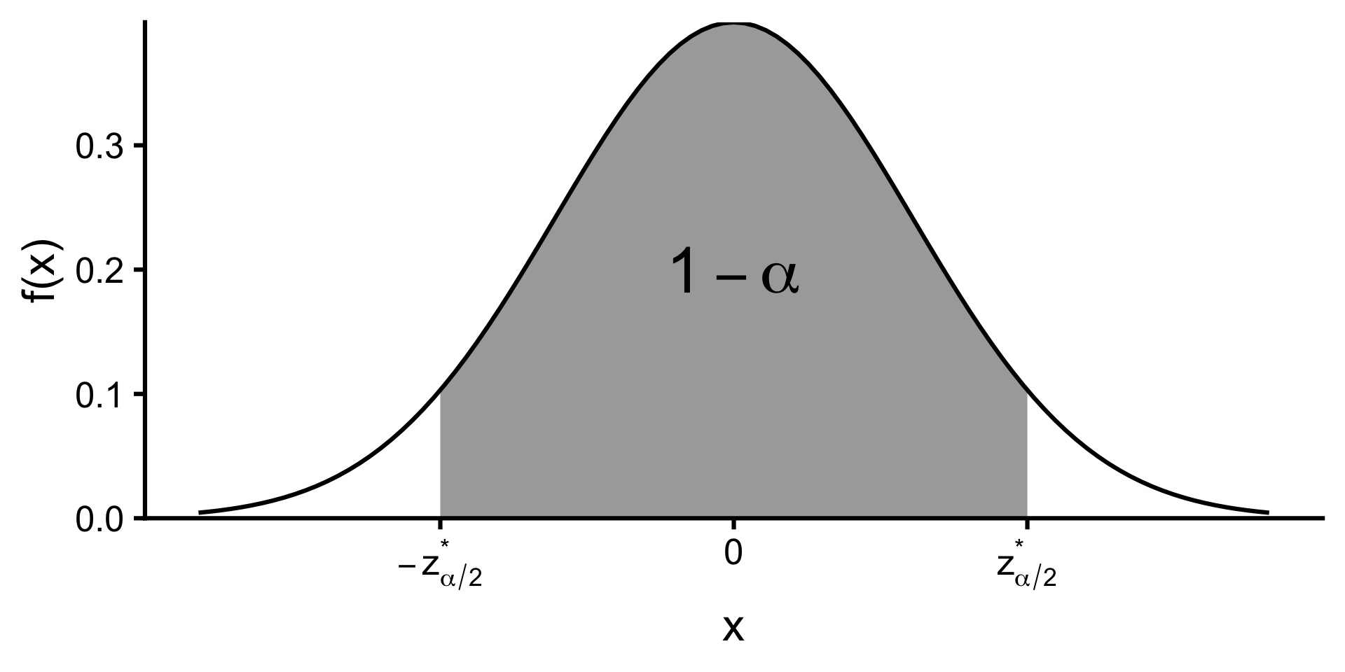
\[\left(\bar{X}-z^*_{\alpha/2}\frac{\sigma}{\sqrt{n}},\;\bar{X}+z^*_{\alpha/2}\frac{\sigma}{\sqrt{n}}\right)\]

where \(z^*_{\alpha/2}\) is the critical value such that \[P(Z < z^*_{\alpha/2}) = 1 - \alpha/2\] for \(Z \sim N(0,1)\).

Interpretation of confidence intervals

Suppose we repeat the experiment many times and construct a \(100(1 - \alpha)\%\) confidence interval from each sample. We expect that approximately \(100(1 - \alpha)\%\) of those intervals will contain the true parameter value.

The parameter \(\mu\) is fixed (in the frequentist paradigm).
The interval is random.
The confidence interval is not a probability statement about the parameter being in the interval.
It is a statement about the long-run performance of the method used to construct the interval.
The interval either contains the parameter or it does not.

Simulating confidence intervals when \(\sigma\) is known

Visualising confidence intervals when \(\sigma\) is known

Factors affecting the width of a confidence interval

Sample size: Larger \(n\) → narrower interval.
Confidence level: Higher confidence → wider interval.
Population variability: More variability → wider interval.

\[\left(\bar{X}-z^*_{\alpha/2}\frac{\sigma}{\sqrt{n}},\;\bar{X}+z^*_{\alpha/2}\frac{\sigma}{\sqrt{n}}\right)\]

A \(100(1 - \alpha)\%\) confidence interval for \(\mu\) when \(\sigma\) is unknown

Population standard deviation usually unknown.
When \(\sigma\) is estimated with the sample standard deviation \(s\):

\[ \frac{\bar{X}-\mu}{s/\sqrt{n}} \sim t_{n-1} \]

\[ \left( \bar{X}-t^*_{n-1,\alpha/2}\frac{s}{\sqrt{n}},\; \bar{X}+t^*_{n-1,\alpha/2}\frac{s}{\sqrt{n}} \right) \]

where \(t^*_{n-1,\alpha/2}\) is the critical value such that \[P(T < t^*_{n-1,\alpha/2}) = 1 - \alpha/2\] for \(T \sim t_{n-1}\).

Simulating confidence intervals when \(\sigma\) is unknown

Does it really make a difference if you use the t-distribution instead of the normal distribution when \(\sigma\) is unknown? Let’s find out by simulating confidence intervals using both methods.

Example: electricity usage

A random sample of 30 households was selected as part of a study on electricity usage, and the number of kilowatt-hours (kWh) was recorded for each household in the sample for the March quarter of 2006. The average usage was found to be 375kWh sample standard deviation is 91.5kWh. Find a 99% confidence interval for the mean usage in the March quarter of 2006.

First, write what you know: \(n = 30\), \(\bar{x} = 375\), \(s = 91.5\), confidence level = 99% \(\Rightarrow \alpha = 0.01\).
Check conditions: sampling distribution of \(\bar{X}\) is approximately normal since \(n\) is large enough.
Since \(\sigma\) is unknown, the critical value is given by \(t^*_{29, 0.005}\) and the standard error is \(s/\sqrt{n}\).

Confidence intervals for a population proportion

Confidence interval for a population proportion

Recall that from CLT that if we have \(X \sim B(n, p)\), then \[\hat{p} = X/n \overset{\text{approx.}}{\sim} N\left(p, \frac{p(1-p)}{n}\right)\] when \(n\) is large enough.
Check the success-failure condition: \(np \geq 10\) and \(n(1-p) \geq 10\).

A \(100(1 - \alpha)\%\) confidence interval for \(p\) is given by

\[\left(\hat{p} - z^*_{\alpha/2}\sqrt{\frac{\hat{p}(1-\hat{p})}{n}},\;\hat{p} + z^*_{\alpha/2}\sqrt{\frac{\hat{p}(1-\hat{p})}{n}}\right)\]

Example: vaccine

A random sample of 100 preschool children in Bruce revealed that only 62 had been vaccinated. Provide an approximate 90% confidence interval for the proportion vaccinated in that suburb.

We have \(n = 100\), \(\hat{p} = 0.62\), confidence level = 90% \(\Rightarrow \alpha = 0.1\).
Check conditions: \(np = 62 \geq 10\) and \(n(1-p) = 38 \geq 10\).
The critical value is \(z^*_{0.05}\) and the standard error is \(\sqrt{\hat{p}(1-\hat{p})/n}\).

Summary

A \((1 - \alpha)100\%\) confidence interval for the mean \(\mu\) is of the form:

\[\text{Point Estimate} \pm \text{Critical Value} \times \text{Standard Error of Point Estimate}.\]

When \(\sigma\) is known: \(\bar{X} \pm z^*_{\alpha/2}\dfrac{\sigma}{\sqrt{n}}\)
- where \(z^*_{\alpha/2}\) is the critical value such that \(P(Z < z^*_{\alpha/2}) = 1 - \alpha/2\) for \(Z \sim N(0,1)\).
When \(\sigma\) is unknown: \(\bar{X} \pm t^*_{n-1,\alpha/2}\dfrac{S}{\sqrt{n}}\)
- where \(t^*_{n-1,\alpha/2}\) is the critical value such that \(P(T < t^*_{n-1,\alpha/2}) = 1 - \alpha/2\) for \(T \sim t_{n-1}\).
For a population proportion: \(\hat{p} \pm z^*_{\alpha/2}\sqrt{\dfrac{\hat{p}(1-\hat{p})}{n}}\)