Advanced R Programming

STAT1003 – Statistical Techniques

Dr. Emi Tanaka

Australian National University

These slides are best viewed on a modern browser like Google Chrome on a desktop or laptop. Some interactive components may require some time to fully load.

Not examinable

Please note that this content is not examinable. It is meant to be a demonstration of how to use R for simulation studies and functional programming, which are useful skills for data analysis but not directly assessed in the course.

Functional Programming

Repetitive tasks

🎯 Let’s calculate the number of distinct values for each column and store it in n

Anything you notice from above?

Using for loops

But R is notoriously known for being slow using for loops

The across function in dplyr can do this without for loops

Note that the result is a data.frame

Functions in R

Functions can be broken into three components:
- formals(), the list of arguments,
- body(), the code inside the function, and
- environment()¹.
Functions in R are created using function() with binding to a name using <- or =

Function body

The body of a function can be a single expression or a block of code enclosed in {}.

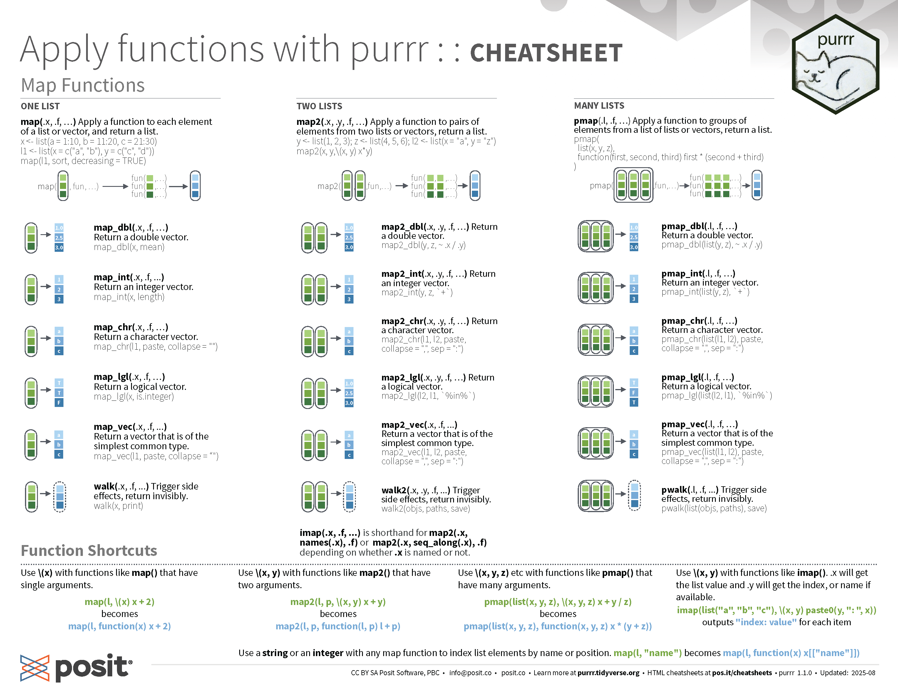
Functional programming with `purrr`

purrr is part of the core tidyverse packages.
It contains a series of map and walk functions.

The related functions in purrr have been design so that that input are consistent.
The user is required to think of the expected output before seeing the output.

`map` functions in `purrr`

map(.x, .f, ...) returns a list
map_chr(.x, .f, ...) returns a vector of character
map_dbl(.x, .f, ...) returns a vector of numeric
map_int(.x, .f, ...) returns a vector of integer
map_lgl(.x, .f, ...) returns a vector of logical

Conditional maps in `purrr`

map_if(.x, .p, .f, ...) uses .p to determine if .f will be applied to .x
map_at(.x, .at, .f, ...) applies .f to .x at .at (name or position)
map_depth(.x, .depth, .f, ...) apples .f to .x at a specific depth level of a nested vector
The return object is always a list

Functional programming in Base R

lapply, Map, mapply, sapply, tapply, apply, and vapply are variants of functional programming in Base R

Some function outputs in Base R are more predictable than others:
- purrr::map is a variant of lapply (which always returns list)
- purrr::pmap is a variant of Map (which takes more than one input)
sapply doesn’t require users to specify the output type, instead it’ll try to figure out what looks best for the user… great for interactive use but require great caution for programming

Anonymous functions

Anonymous functions, also called lambda expression in computer programming, are functions without names.

Since R version 4.1.0, we can use the shorthand \(x) to define anonymous functions

Tidyverse employs a special shorthand using a formula and .x as a special placeholder for input

Formula anonymous function in Tidyverse

Formula anonymous functions are not just for purrr functions:

Most tidyverse functions would support this formula approach to anonymous function, but likely not outside of that ecosystem unless developers adopt the same system.

Functions with two inputs

For functions with two inputs, you can use the map2 variants in purrr

For anonymous functions with two inputs, the first input is .x (as before) and the second is .y

Functions with more than two inputs

What about if there are more than two input?
You can use pmap variants in purrr

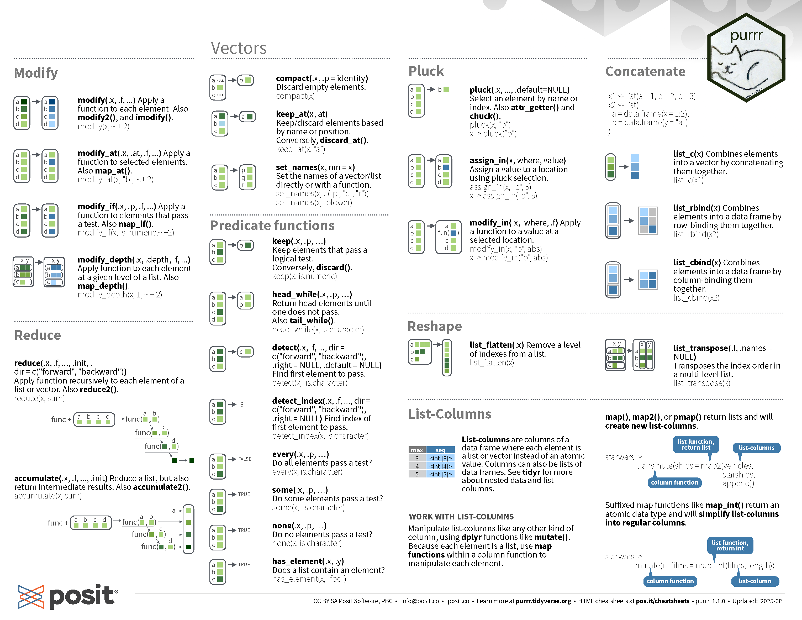
Other functions in `purrr`

Using names of input

The imap(x) variants are shorthand for map2(x, names(x))

Expecting no return object

If you are looking to get a side effect rather than return, you can use the walk variants

`reduce` function in `purrr`

reduce(.x, .f) applies a function .f cumulatively to the elements of .x, from left to right.
E.g. reduce(c(1, 2, 3, 4), sum) is equivalent to sum(sum(sum(1, 2), 3), 4)

accumulate(.x, .f) is similar to reduce, but it returns the intermediate results as well.

`purrr` cheatsheet

Simulation Design

Simulation study

Simulation is a powerful tool to understand the behaviour of a system when we cannot easily derive the answer mathematically.
In a simulation study, we need:
- a data generating process (DGP) that mimics the real-world process we are interested in, and
- a statistic that we want to study the behaviour of.

Simulation design

We can consider various scenarios or factors that may affect the behaviour of the statistic.
We can then use simulation to explore how the statistic behaves under different scenarios.

Rolling 10 dices

Let \(X\) be the total of rolling 10 dice.
We can get the exact distribution of \(X\) by enumerating all possible outcomes of rolling 10 dice, and counting the number of outcomes that give each possible total.

Alternative approach

This requires more memory, as it needs to store all possible outcomes of rolling 10 dice, which is \(6^{10} = 60,466,176\) outcomes. However, it is more straightforward to implement and understand.

Simulate rolling 10 dice

We can also simulate rolling 10 dice by generating random numbers from a (discrete) uniform distribution and summing them up.

Rolling 10,000 dices

Let \(X\) be the total of rolling 10,000 dice.
Suppose we want to know the probability that \(X\) is greater than 35,000.
We can use the exact distribution approach, but it is computationally infeasible as it requires enumerating all possible outcomes of rolling 10,000 dice, which is \(6^{10000}\) outcomes.
However, we can easily simulate rolling 10,000 dice and estimate the probability that \(X\) is greater than 30,000.

Bootstrapping

Bootstrapping is frequently used to estimate the sampling distribution of a statistic when the underlying population distribution is unknown or when the sample size is small.
The bootstrap method involves repeatedly resampling with replacement from the observed data and calculating the statistic of interest for each resample.

Summary

Simulation is a powerful tool to understand the behaviour of a system when we cannot easily derive the answer mathematically.
In a simulation study, we need a data generating process (DGP) that mimics the real-world process we are interested in, and a statistic that we want to study the behaviour of.
We can consider various scenarios or factors that may affect the behaviour of the statistic, and use simulation to explore how the statistic behaves under different scenarios.
Simulation can be used to estimate probabilities or other characteristics of a statistic when the exact distribution is computationally infeasible to derive.
Bootstrapping is a resampling method that can be used to estimate the sampling distribution of a statistic when the underlying population distribution is unknown or when the sample size is small.