Acknowledgement

This lecture was partially adapted from the previous STAT1003 lecturers. Thank you folks!

Continuous random variables

Continuous random variable

  • A continuous random variable is a random variable that can take on an infinite number of values within a given range.
  • The probability density function (pdf) for a continuous random variable is not defined in the same way as for a discrete random variable.
  • It is impossible to assign a non-zero probability to any single point for a continuous random variable, because there are infinitely many possible values that the variable can take on.
  • For the wheel spinner example, what is the probability that the pointer lands on
    • exactly 180 degrees?
    • exactly 180.000001 degrees?
    • exactly 180.0000000000000001 degrees?
  • Let \(X\) be the degrees clockwise from the pointer to the black edge.
  • \(X\) is any value in \([0, 360)\) with a specific range of values being equally likely.

Computing probabilities for continuous random variables

  • For a continuous random variable \(X\), any value \(x\): \[P(X = x) = 0.\]
  • Instead of assigning probabilities to individual points, we assign probabilities to intervals \((a, b)\), \[P(a < X < b).\]
  • For the wheel spinner example, \(P(0 < X < 180) = 0.5\) (why?)
  • Discrete: there are some \(x\) where \(P(X\leq x) \neq P(X < x)\)
  • Continuous: for any \(x\), \(P(X \leq x) = P(X < x)\)

Empirical probability distribution

  • Column Area \(=\) Interval Width \(\times\) Column Height
  • Column Area \(=\) Proportion
  • Column Height \(=\) Proportion / Interval Width
  • We call this column height as density
  • The sum of all column areas add up to 1.

0.0005 + 0.1741 + 0.5780 + 0.2411 + 0.0064 \(\approx\) 1


For large sample size and small bin width, the histogram approximates the probability density function of the population distribution.

Probability density function

  • The pdf, \(f_X(x)\), of a continuous random variable \(X\) must satisfy:
    • \(f_X(x) \geq 0\) for all \(x\) (non-negative).
    • \(\int_{-\infty}^\infty f_X(x)dx = 1\) (total area under curve equals 1).
  • The probability that \(X\) lies between \(a\) and \(b\) is equal to area under the pdf between the points \(a\) and \(b\):

\[P(a < X < b) =\int_a^b f_X(x)dx.\]


Finding probabilities using the pdf

Consider the function

\[f_X(x) = \begin{cases} 4x & \text{for } 0 < x < 0.5 \\ 4 - 4x & \text{for } 0.5 \leq x < 1 \\ 0 & \text{otherwise} \end{cases}\]

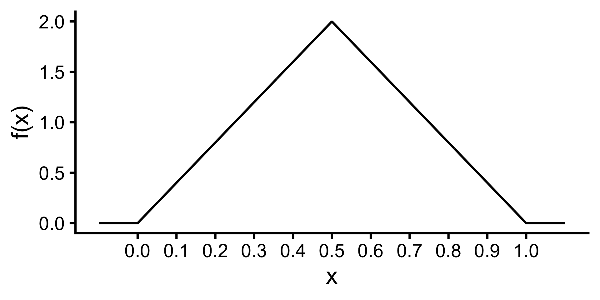
  • Is \(f_X(x)\) a valid pdf?
  • What is \(P(0.2 < X < 0.3)\) where \(X\) is a random variable with pdf \(f_X(x)\)?

Expected value

The expected value (or population mean) of a continuous random variable \(X\) is defined to be: \[\mu = E(X) = \int_{-\infty}^\infty xf_X(x)dx.\]

  • The expected value of \(g(X)\), where \(g(X)\) is some function of \(X\), is defined to be: \[E(g(X)) = \int_{-\infty}^\infty g(x)f(x)dx.\]

\[\begin{align*} E(X) &= \int_{-\infty}^\infty xf_X(x)dx\\ &= \int_0^{0.5} 4x^2 dx + \int_{0.5}^1 x(4 - 4x) dx\\ &= 4 \times \frac{0.5^3}{3} + 4 \times \left(\frac{1^2}{2} - \frac{0.5^2}{2}\right) \\ &\quad - 4 \times \left(\frac{1^3}{3} - \frac{0.5^3}{3}\right)\\ &= 0.5 \end{align*}\]

Variance

The (population) variance of a continuous random variable \(X\) is defined to be: \[\sigma^{2}=\text{Var}(X)=E\left((X-\mu)^{2}\right)=\int_{-\infty}^{\infty}(x-\mu)^{2} f_X(x) d x.\]

  • A shortcut formula for the variance is given below:

\[\text{Var}(X)=E\left(X^{2}\right)-(E(X))^{2}=\left(\int_{-\infty}^{\infty} x^{2} f(x) d x\right)-\mu^{2}\]

  • The standard deviation is \(SD(X) = \sigma = \sqrt{\text{Var}(X)}\)

Cumulative distribution function

  • The cumulative distribution function (cdf) for a random variable \(X\) is defined to be \[F_X(x) = P(X\leq x).\]
  • For a continuous random variable with pdf \(f_X\) \[F_X(x) = \int_{-\infty}^x f_X(t)dt\]
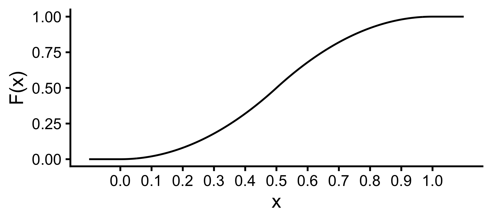
pdf \[f_X(x) = \begin{cases} 4x & \text{for } 0 < x < 0.5 \\ 4 - 4x & \text{for } 0.5 \leq x < 1 \\ 0 & \text{otherwise} \end{cases}\]

The cdf is given by

\[F_X(x) = \begin{cases} 0 & \text{for } x \leq 0 \\ 2x^2 & \text{for } 0 < x < 0.5 \\ 4x - 2x^2 - 1 & \text{for } 0.5 \leq x < 1 \\ 1 & x \geq 1 \end{cases}\]

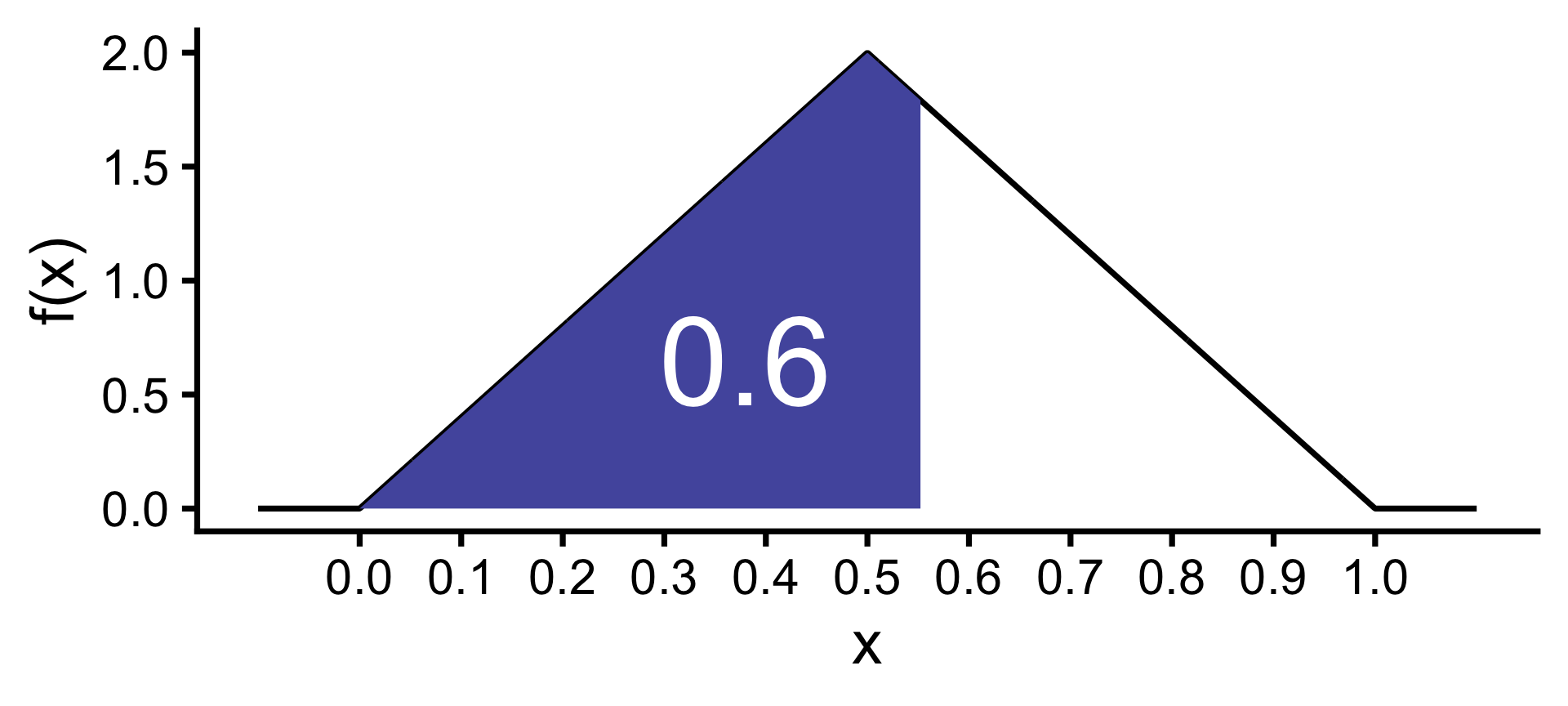
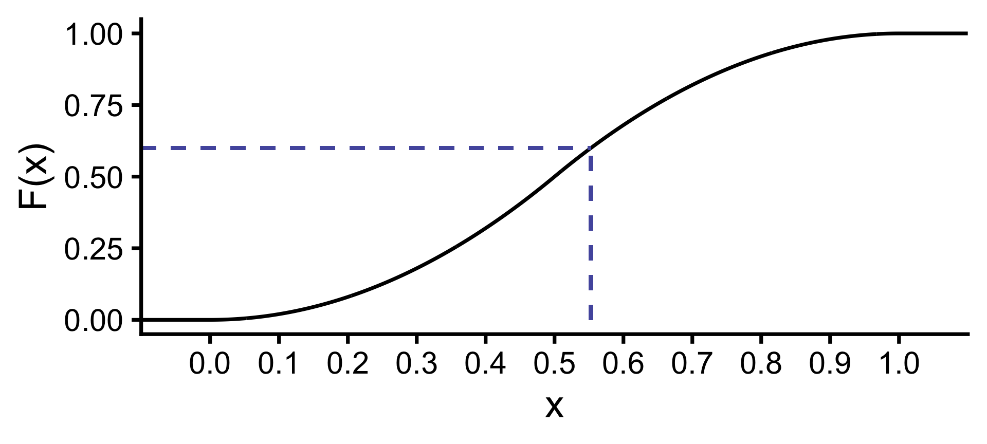
Quantiles with probability distributions

For a distribution with a pdf \(f_X(x)\), what is the 60-th percentile?

  • We want to find the value \(q\) such that 60% of population values are below it, i.e. \[P(X\leq q) = 0.6.\]
  • In other words, we want to find \(q\) such that \[\int_{-\infty}^q f_X(x)dx = F(q) = 0.6.\]

\[q \approx 0.553\]

Summary

  • A continuous random variable is a random variable that can take on any value within a certain range or interval.
  • For a continuous random variable \(X\):
    • probability density function (pdf) \(f_X\) must satisfy two properties: (1) \(f_X(x) \geq 0\) for all \(x\), and (2) \(\int_{-\infty}^\infty f_X(x)dx = 1\).
    • \(P(a < X < b) =\int_a^b f_X(x)dx.\)
    • \(\mu = E(X) = \int_{-\infty}^\infty xf_X(x)dx.\)
    • \(E(g(X)) = \int_{-\infty}^\infty g(x)f(x)dx.\)
    • \(\text{Var}(X)=E\left(X^{2}\right)-(E(X))^{2}=\left(\int_{-\infty}^{\infty} x^{2} f(x) d x\right)-\mu^{2}\)
    • The cumulative distribution function (cdf) \(F_X(x) = P(X\leq x)\) is given by \(F_X(x) = \int_{-\infty}^x f_X(t)dt\).
    • The \(p\)-th percentile of a distribution with pdf \(f_X(x)\) is the value \(q\) such that \(\int_{-\infty}^q f_X(x)dx = F(q) = p/100.\)

Continuous parameteric distributions

Continuous data in the wild

Parametric distributions for continuous data

There are a number of special continuous distributions like:

Uniform distribution

Normal distribution \(N(0, 1)\)

t distribution \(N(0, 1)\)


F distribution

Chi-square distribution


Uniform distribution

Uniform distribution

  • A continuous random variable \(X\) is said to have a uniform distribution over the interval \([a,b]\) if its pdf is given by \[ f_X(x)=\left\{\begin{array}{ll} \dfrac{1}{b-a}, & a \leq x\leq b \\ 0, & x < a \text{ or } x>b \end{array}\right. \]

  • We use the notation \(X\sim U(a,b)\) and

  • \(E(X) = \frac{a+b}{2}\)

  • \(\text{Var}(X) = \frac{(b-a)^2}{12}\)

  • Let \(X\) be the degrees clockwise from the pointer to the black edge.
  • \(X \sim U(0, 360)\)

Normal distribution

Normal distribution

  • A continuous random variable \(X\) has a normal distribution if its pdf is: \[f(x; \mu, \sigma) = \frac{1}{\sigma\sqrt{2\pi}}\text{exp}\left(-\frac{(x - \mu)^2}{2\sigma^2}\right)\]

  • Written as \(X \sim N(\mu, \sigma^2)\) where

    • \(E(X) = \mu\)
    • \(\text{Var}(X) = \sigma^2\)
  • \(Z = \dfrac{X - \mu}{\sigma} \sim N(0, 1)\) is referred to as the standard normal distribution.

Total area under the curve = 1.

  • Also referred to as the Gaussian distribution.
  • Distribution is symmetric and bell-shaped.

Z-scores

  • The Z-score is defined as the number of standard deviations a value is from the mean, i.e. \[Z = \frac{X - \mu}{\sigma}.\]

  • Z-scores are used to standardise values from different normal distributions, allowing us to compare them on a common scale.

  • The distribution of SAT and ACT scores are both approximately normal, but they have different means and standard deviations.
  • SAT scores have a mean of 1100 and a standard deviation of 200.
  • ACT scores have a mean of 21 and a standard deviation of 6.
  • Suppose Ann scored 1300 on the SAT and Tom scored 24 on the ACT.
  • Who performed better relative to their peers?

Comparing between normal distributions

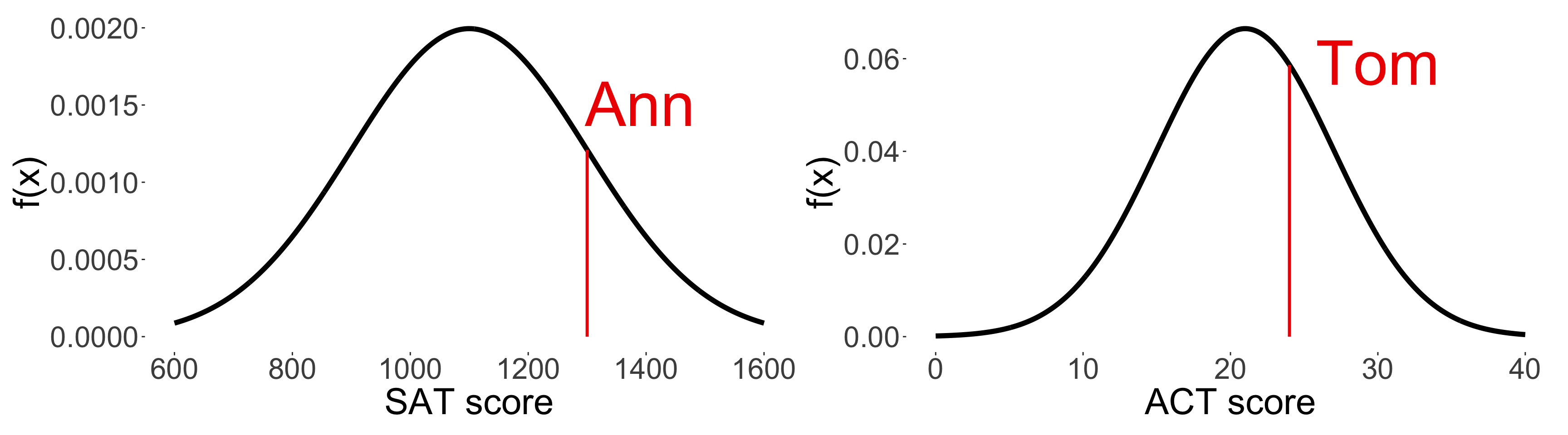
\(z_\text{Ann} = \frac{1300 - 1100}{200} = 1\) and \(z_\text{Tom} = \frac{24 - 21}{6} \approx 0.5\).


\(z_\text{Ann} > z_\text{Tom}\), so Ann performed better relative to her peers than Tom!

Normal distribution in R

\(f_X(x) = \frac{1}{\sigma\sqrt{2\pi}}\text{exp}\left(-\frac{(x - \mu)^2}{2\sigma^2}\right)\) where \(X \sim N(\mu, \sigma^2)\)

\(F_X(x) = \int_{-\infty}^{x} \frac{1}{\sigma\sqrt{2\pi}}\text{exp}\left(-\frac{(t - \mu)^2}{2\sigma^2}\right) \, dt\) where \(X \sim N(\mu, \sigma^2)\)

Find \(q\) such that \(P(X < q) = p\) where \(X \sim N(\mu, \sigma^2)\)

Simulate draws from \(X \sim N(\mu, \sigma^2)\)

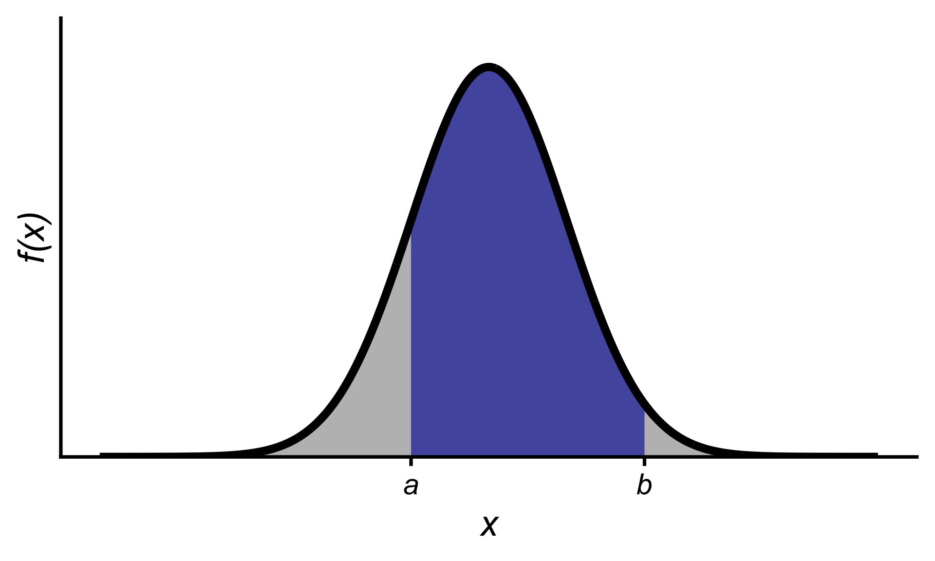
Probability calculation for normal distributions

Recall: the probability of a continuous random variable falling in a specific range is the area under the curve.

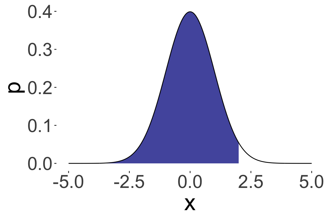
\(P(X < 2)\) where \(X \sim N(0, 1)\)

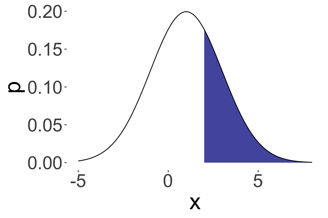
\(P(X > 2)\) where \(X \sim N(1, 2)\)

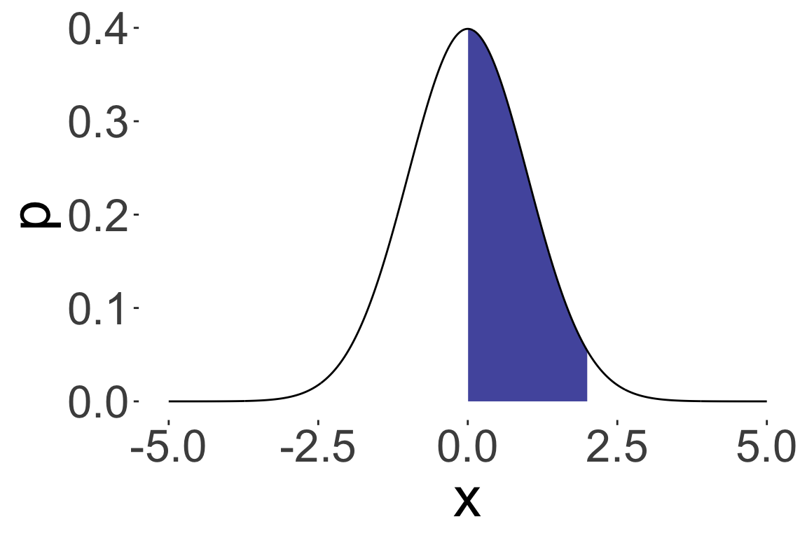
\(P(0 < X < 2)\) where \(X \sim N(0, 1)\)

Using standardisation and symmetry

Suppose that you are given the following R output:

pnorm(c(0, 0.5, 1, 1.5, 2, 2.5, 3))
[1] 0.5000000 0.6914625 0.8413447
[4] 0.9331928 0.9772499 0.9937903
[7] 0.9986501

Using the above information only, calculate the following probabilities:

  • \(P(Z < -1)\) where \(Z \sim N(0, 1)\)
  • \(P(X > 1.5)\) where \(X \sim N(1, 1)\)
  • \(P(|X - 1| > 2)\) where \(X \sim N(1, 2)\)
  • If \(X \sim N(\mu, \sigma^2)\), then \[P(X < a) = P\left(Z < \frac{a - \mu}{\sigma}\right)\] where \(Z \sim N(0, 1)\).
  • The normal distribution is symmetric about its mean, i.e. \[P(X < \mu - a) = P(X > \mu + a)\] for any \(a > 0\).

68-95-99.7 rule

  • For a normal distribution, approximately
    • 68% of the population values are within 1 standard deviation of the mean,
    • 95% are within 2 standard deviations of the mean, and
    • 99.7% are within 3 standard deviations of the mean.


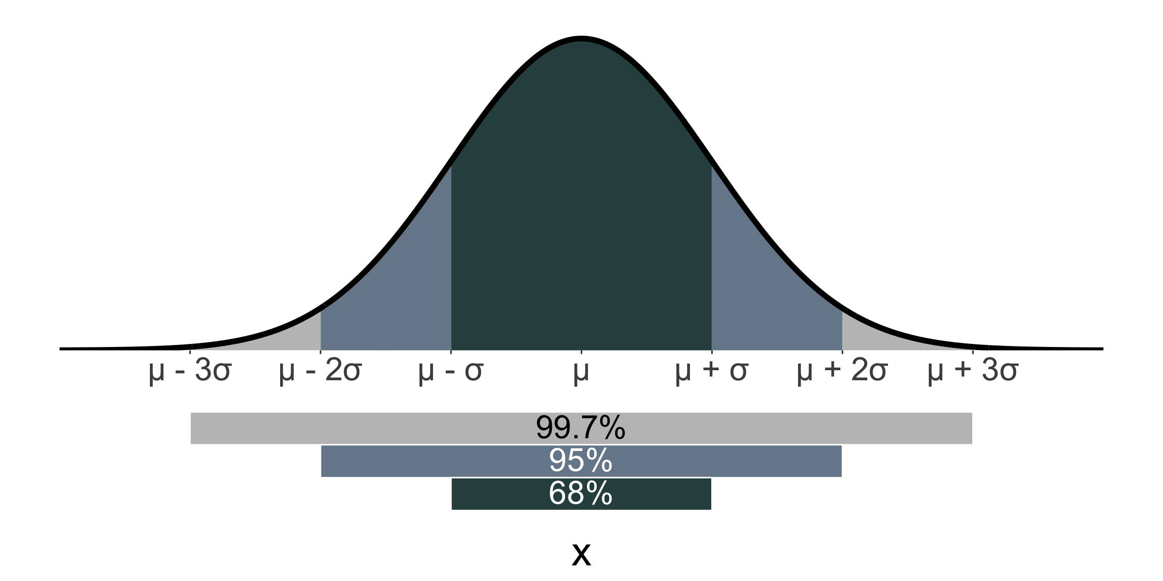
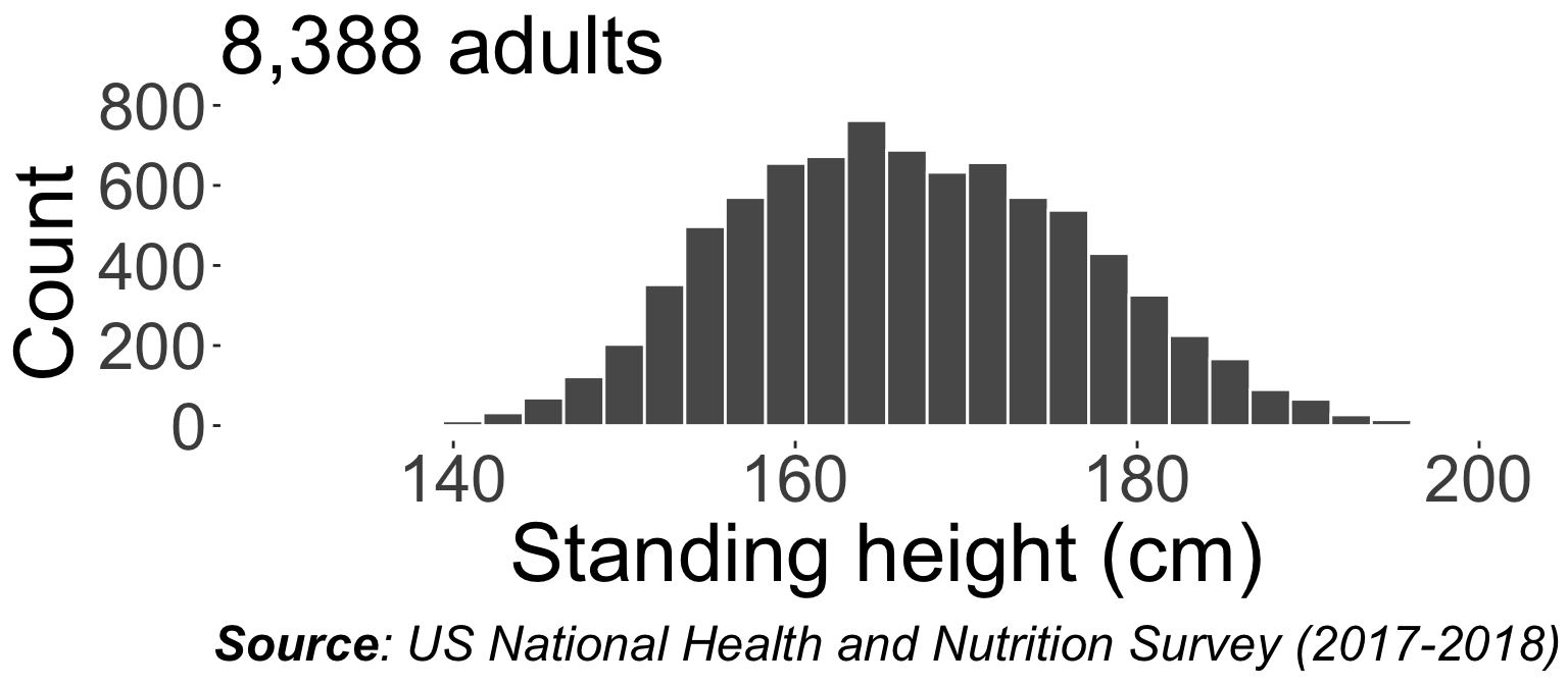
E.g. the average adult height is ~167cm, and the standard deviation is ~10cm based on US National Health and Nutrition Examination Survey (2017-2018) data. So assuming the distribution of adult heights is normal, approximately 99.7% of adults have a height between 137cm and 197cm.

Fitting a normal distribution to data

scroll

  • Standing height (in cm) from the US National Health and Nutrition Examination Survey (2017-2018) data.

Student’s t distribution

Student’s t distribution

  • The t-distribution is a continuous distribution that is symmetric and bell-shaped, but has heavier tails than the standard normal distribution.
  • The t-distribution is used when the sample size is small and the population standard deviation is estimated from the sample.
  • The grey area is \(N(0, 1)\) for comparison.
  • As the degrees of freedom increases, the t-distribution approaches the standard normal distribution.
  • \(X \sim t_\nu\) where \(\nu\) is the degrees of freedom.
  • \(E(X) = 0\) for \(\nu > 1\).
  • \(Var(X) = \dfrac{\nu}{\nu - 2}\) for \(\nu > 2\).

t-distribution in R

  • The t-distribution is implemented in R using the dt(), pt(), qt(), and rt() functions, which are analogous to the dnorm(), pnorm(), qnorm(), and rnorm() functions for the normal distribution.

  • When the sample size is large, there is not much difference:

  • However, when the sample size is small, the t-distribution gives a different result:

Summary

Distribution Support Mean Variance
\(X \sim U(a, b)\) \([a, b]\) \(\dfrac{a + b}{2}\) \(\dfrac{(b - a)^2}{12}\)
\(X \sim N(\mu, \sigma^2)\) \((-\infty, \infty)\) \(\mu\) \(\sigma^2\)
\(X \sim t(\nu)\) \((-\infty, \infty)\) \(0\) (for \(\nu > 1\)) \(\frac{\nu}{\nu - 2}\) (for \(\nu > 2\))
Distribution pdf cdf quantile function random generation
Uniform dunif(x, a, b) punif(q, a, b) qunif(p, a, b) runif(n, a, b)
Normal dnorm(x, mean, sd) pnorm(q, mean, sd) qnorm(p, mean, sd) rnorm(n, mean, sd)
t-distribution dt(x, df) pt(q, df) qt(p, df) rt(n, df)
  • The normal distribution is a continuous distribution that is symmetric and bell-shaped, and is used to model many natural phenomena.
  • The t-distribution has heavier tails than the standard normal distribution, and is used when the sample size is small and the population standard deviation is estimated from the sample.