Continuous Random Variables

STAT1003 – Statistical Techniques

Dr. Emi Tanaka

Australian National University

These slides are best viewed on a modern browser like Google Chrome on a desktop or laptop. Some interactive components may require some time to fully load.

Table of contents

• Continuous random variable
• Computing probabilities for continuous random variables
• Empirical probability distribution
• Probability density function
• Finding probabilities using the pdf
• Expected value
• Variance
• Cumulative distribution function
• Quantiles with probability distributions
• Summary

Continuous random variable

• A continuous random variable is a random variable that can take on an infinite number of values within a given range.
• The probability density function (pdf) for a continuous random variable is not defined in the same way as for a discrete random variable.
• It is impossible to assign a non-zero probability to any single point for a continuous random variable, because there are infinitely many possible values that the variable can take on.
• For the wheel spinner example, what is the probability that the pointer lands on
  • exactly 180 degrees?
  • exactly 180.000001 degrees?
  • exactly 180.0000000000000001 degrees?

• Let \(X\) be the degrees clockwise from the pointer to the black edge.
• \(X\) is any value in \([0, 360)\) with a specific range of values being equally likely.

Computing probabilities for continuous random variables

• For a continuous random variable \(X\), any value \(x\): \[P(X = x) = 0.\]
• Instead of assigning probabilities to individual points, we assign probabilities to intervals \((a, b)\), \[P(a < X < b).\]
• For the wheel spinner example, \(P(0 < X < 180) = 0.5\) (why?)

• Discrete: there are some \(x\) where \(P(X\leq x) \neq P(X < x)\)
• Continuous: for any \(x\), \(P(X \leq x) = P(X < x)\)

Empirical probability distribution

• Column Area \(=\) Interval Width \(\times\) Column Height
• Column Area \(=\) Proportion
• Column Height \(=\) Proportion / Interval Width
• We call this column height as density
• The sum of all column areas add up to 1.

0.0005 + 0.1741 + 0.5780 + 0.2411 + 0.0064 \(\approx\) 1

For large sample size and small bin width, the histogram approximates the probability density function of the population distribution.

Probability density function

• The pdf, \(f_X(x)\), of a continuous random variable \(X\) must satisfy:
  • \(f_X(x) \geq 0\) for all \(x\) (non-negative).
  • \(\int_{-\infty}^\infty f_X(x)dx = 1\) (total area under curve equals 1).
• The probability that \(X\) lies between \(a\) and \(b\) is equal to area under the pdf between the points \(a\) and \(b\):

\[P(a < X < b) =\int_a^b f_X(x)dx.\]

Finding probabilities using the pdf

Consider the function

\[f_X(x) = \begin{cases} 4x & \text{for } 0 < x < 0.5 \\ 4 - 4x & \text{for } 0.5 \leq x < 1 \\ 0 & \text{otherwise} \end{cases}\]

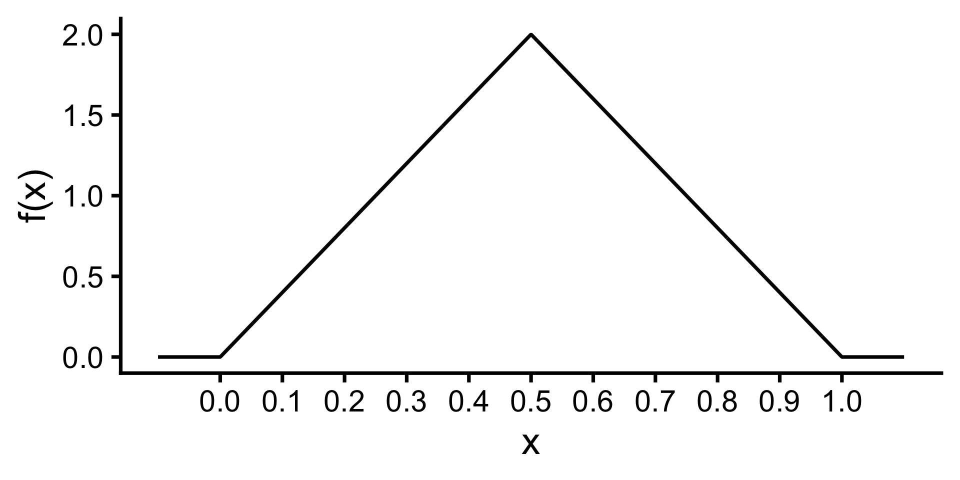
• Is \(f_X(x)\) a valid pdf?
• What is \(P(0.2 < X < 0.3)\) where \(X\) is a random variable with pdf \(f_X(x)\)?

Expected value

The expected value (or population mean) of a continuous random variable \(X\) is defined to be: \[\mu = E(X) = \int_{-\infty}^\infty xf_X(x)dx.\]

• The expected value of \(g(X)\), where \(g(X)\) is some function of \(X\), is defined to be: \[E(g(X)) = \int_{-\infty}^\infty g(x)f(x)dx.\]

\[\begin{align*} E(X) &= \int_{-\infty}^\infty xf_X(x)dx\\ &= \int_0^{0.5} 4x^2 dx + \int_{0.5}^1 x(4 - 4x) dx\\ &= 4 \times \frac{0.5^3}{3} + 4 \times \left(\frac{1^2}{2} - \frac{0.5^2}{2}\right) \\ &\quad - 4 \times \left(\frac{1^3}{3} - \frac{0.5^3}{3}\right)\\ &= 0.5 \end{align*}\]

Variance

The (population) variance of a continuous random variable \(X\) is defined to be: \[\sigma^{2}=\text{Var}(X)=E\left((X-\mu)^{2}\right)=\int_{-\infty}^{\infty}(x-\mu)^{2} f_X(x) d x.\]

• A shortcut formula for the variance is given below:

\[\text{Var}(X)=E\left(X^{2}\right)-(E(X))^{2}=\left(\int_{-\infty}^{\infty} x^{2} f(x) d x\right)-\mu^{2}\]

• The standard deviation is \(SD(X) = \sigma = \sqrt{\text{Var}(X)}\)

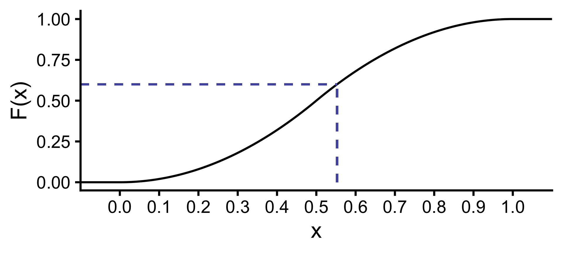
Cumulative distribution function

• The cumulative distribution function (cdf) for a random variable \(X\) is defined to be \[F_X(x) = P(X\leq x).\]
• For a continuous random variable with pdf \(f_X\) \[F_X(x) = \int_{-\infty}^x f_X(t)dt\]

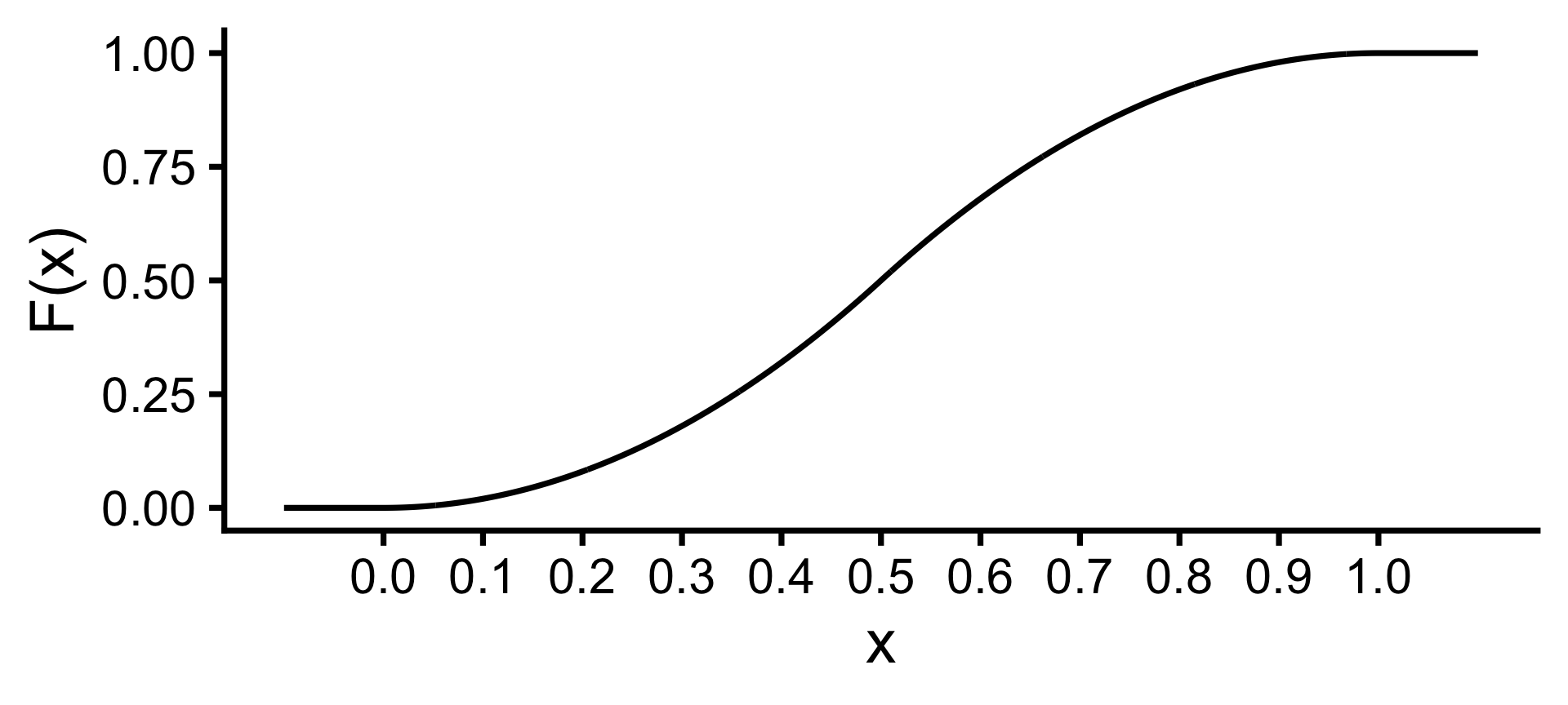
pdf

\[f_X(x) = \begin{cases} 4x & \text{for } 0 < x < 0.5 \\ 4 - 4x & \text{for } 0.5 \leq x < 1 \\ 0 & \text{otherwise} \end{cases}\]

The cdf is given by

\[F_X(x) = \begin{cases} 0 & \text{for } x \leq 0 \\ 2x^2 & \text{for } 0 < x < 0.5 \\ 4x - 2x^2 - 1 & \text{for } 0.5 \leq x < 1 \\ 1 & x \geq 1 \end{cases}\]

Quantiles with probability distributions

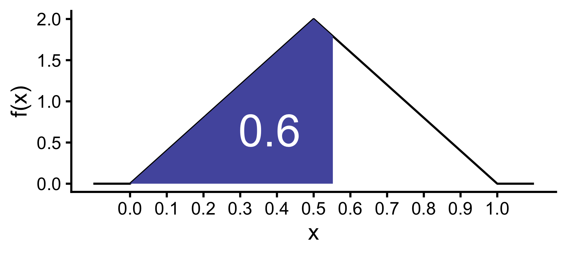
For a distribution with a pdf \(f_X(x)\), what is the 60-th percentile?

• We want to find the value \(q\) such that 60% of population values are below it, i.e. \[P(X\leq q) = 0.6.\]
• In other words, we want to find \(q\) such that \[\int_{-\infty}^q f_X(x)dx = F(q) = 0.6.\]

\[q \approx 0.553\]

Summary

• A continuous random variable is a random variable that can take on any value within a certain range or interval.
• For a continuous random variable \(X\):
  • probability density function (pdf) \(f_X\) must satisfy two properties: (1) \(f_X(x) \geq 0\) for all \(x\), and (2) \(\int_{-\infty}^\infty f_X(x)dx = 1\).
  • \(P(a < X < b) =\int_a^b f_X(x)dx.\)
  • \(\mu = E(X) = \int_{-\infty}^\infty xf_X(x)dx.\)
  • \(E(g(X)) = \int_{-\infty}^\infty g(x)f(x)dx.\)
  • \(\text{Var}(X)=E\left(X^{2}\right)-(E(X))^{2}=\left(\int_{-\infty}^{\infty} x^{2} f(x) d x\right)-\mu^{2}\)
  • The cumulative distribution function (cdf) \(F_X(x) = P(X\leq x)\) is given by \(F_X(x) = \int_{-\infty}^x f_X(t)dt\).
  • The \(p\)-th percentile of a distribution with pdf \(f_X(x)\) is the value \(q\) such that \(\int_{-\infty}^q f_X(x)dx = F(q) = p/100.\)