Continuous parametric distributions

STAT1003 – Statistical Techniques

Dr. Emi Tanaka

Australian National University

These slides are best viewed on a modern browser like Google Chrome on a desktop or laptop. Some interactive components may require some time to fully load.

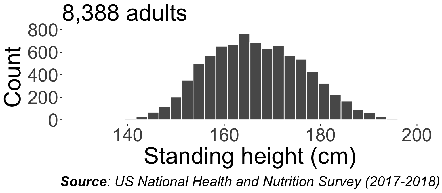
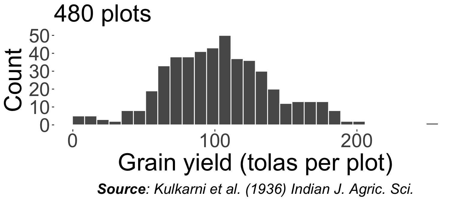
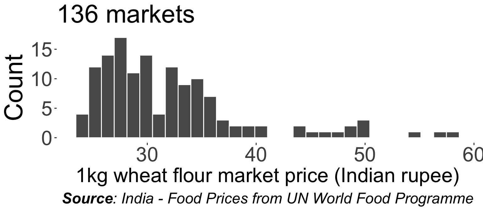
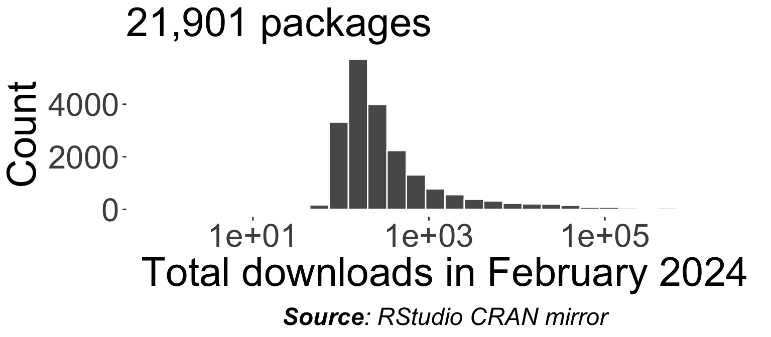
Continuous data in the wild

Parametric distributions for continuous data

There are a number of special continuous distributions like:

Uniform distribution

Normal distribution \(N(0, 1)\)

t distribution \(N(0, 1)\)


F distribution

Chi-square distribution


Uniform distribution

Uniform distribution

  • A continuous random variable \(X\) is said to have a uniform distribution over the interval \([a,b]\) if its pdf is given by \[ f_X(x)=\left\{\begin{array}{ll} \dfrac{1}{b-a}, & a \leq x\leq b \\ 0, & x < a \text{ or } x>b \end{array}\right. \]

  • We use the notation \(X\sim U(a,b)\) and

  • \(E(X) = \frac{a+b}{2}\)

  • \(\text{Var}(X) = \frac{(b-a)^2}{12}\)

  • Let \(X\) be the degrees clockwise from the pointer to the black edge.
  • \(X \sim U(0, 360)\)

Normal distribution

Normal distribution

  • A continuous random variable \(X\) has a normal distribution if its pdf is: \[f(x; \mu, \sigma) = \frac{1}{\sigma\sqrt{2\pi}}\text{exp}\left(-\frac{(x - \mu)^2}{2\sigma^2}\right)\]

  • Written as \(X \sim N(\mu, \sigma^2)\) where

    • \(E(X) = \mu\)
    • \(\text{Var}(X) = \sigma^2\)
  • \(Z = \dfrac{X - \mu}{\sigma} \sim N(0, 1)\) is referred to as the standard normal distribution.

Total area under the curve = 1.

  • Also referred to as the Gaussian distribution.
  • Distribution is symmetric and bell-shaped.

Z-scores

  • The Z-score is defined as the number of standard deviations a value is from the mean, i.e. \[Z = \frac{X - \mu}{\sigma}.\]

  • Z-scores are used to standardise values from different normal distributions, allowing us to compare them on a common scale.

  • The distribution of SAT and ACT scores are both approximately normal, but they have different means and standard deviations.
  • SAT scores have a mean of 1100 and a standard deviation of 200.
  • ACT scores have a mean of 21 and a standard deviation of 6.
  • Suppose Ann scored 1300 on the SAT and Tom scored 24 on the ACT.
  • Who performed better relative to their peers?

Comparing between normal distributions

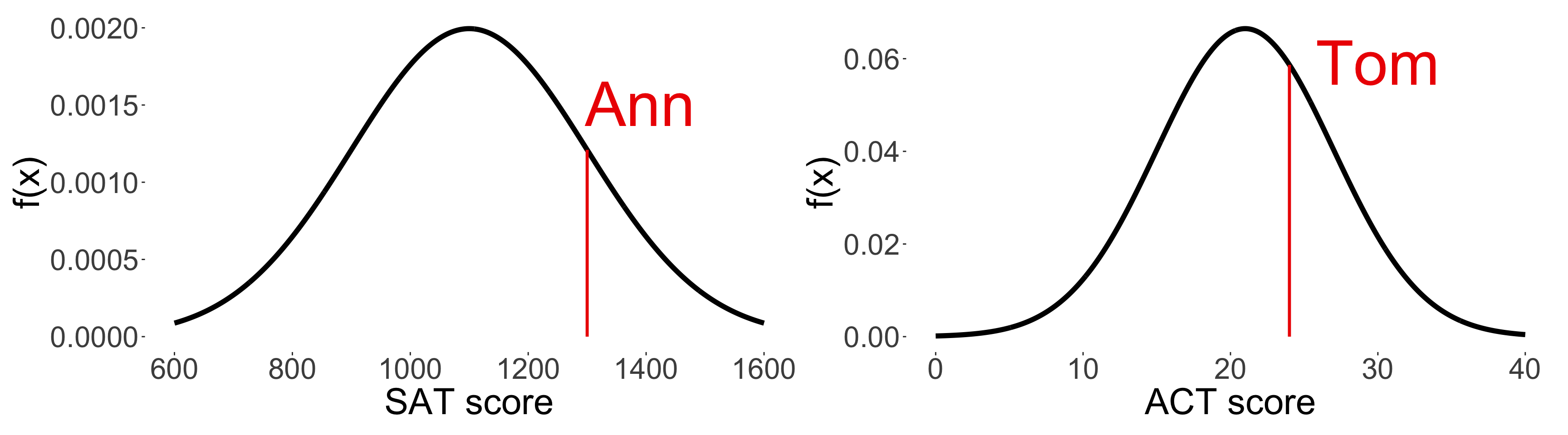
\(z_\text{Ann} = \frac{1300 - 1100}{200} = 1\) and \(z_\text{Tom} = \frac{24 - 21}{6} \approx 0.5\).


\(z_\text{Ann} > z_\text{Tom}\), so Ann performed better relative to her peers than Tom!

Normal distribution in R

\(f_X(x) = \frac{1}{\sigma\sqrt{2\pi}}\text{exp}\left(-\frac{(x - \mu)^2}{2\sigma^2}\right)\) where \(X \sim N(\mu, \sigma^2)\)

\(F_X(x) = \int_{-\infty}^{x} \frac{1}{\sigma\sqrt{2\pi}}\text{exp}\left(-\frac{(t - \mu)^2}{2\sigma^2}\right) \, dt\) where \(X \sim N(\mu, \sigma^2)\)

Find \(q\) such that \(P(X < q) = p\) where \(X \sim N(\mu, \sigma^2)\)

Simulate draws from \(X \sim N(\mu, \sigma^2)\)

Probability calculation for normal distributions

Recall: the probability of a continuous random variable falling in a specific range is the area under the curve.

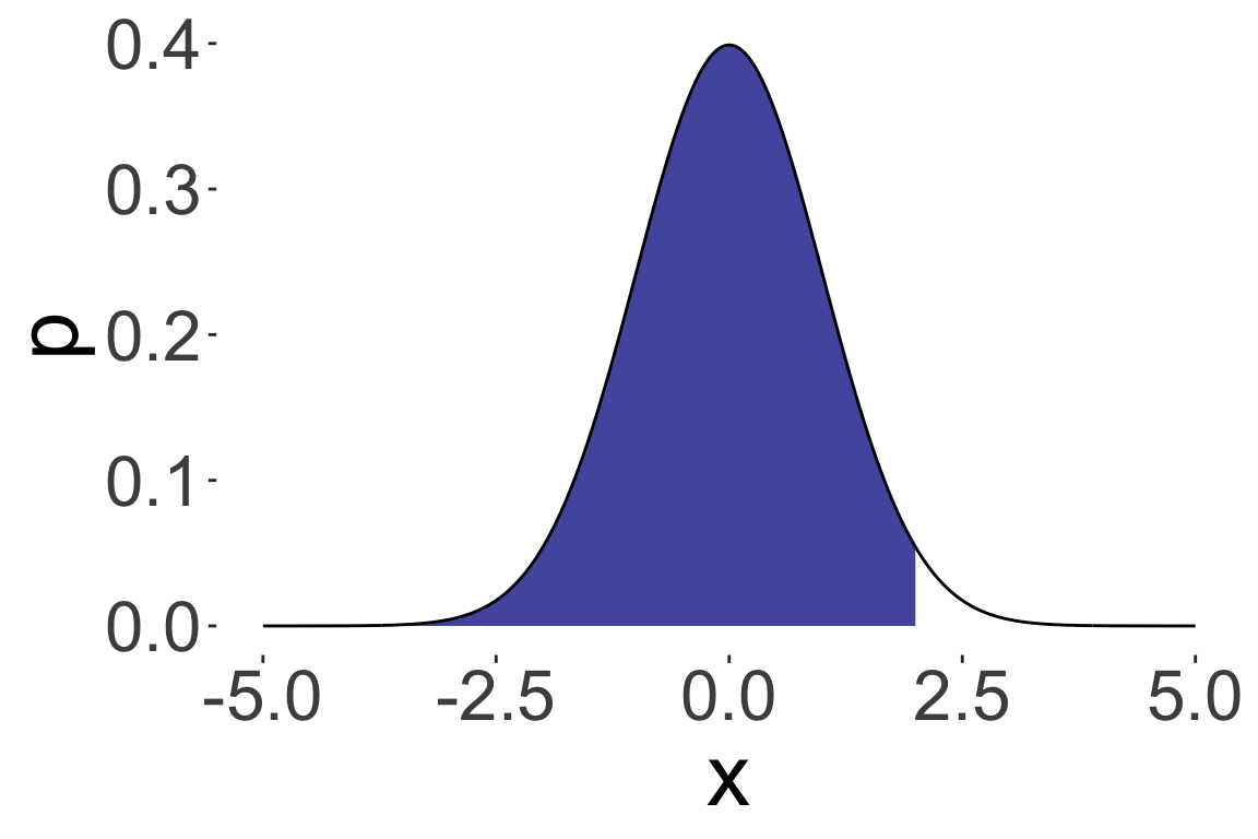
\(P(X < 2)\) where \(X \sim N(0, 1)\)

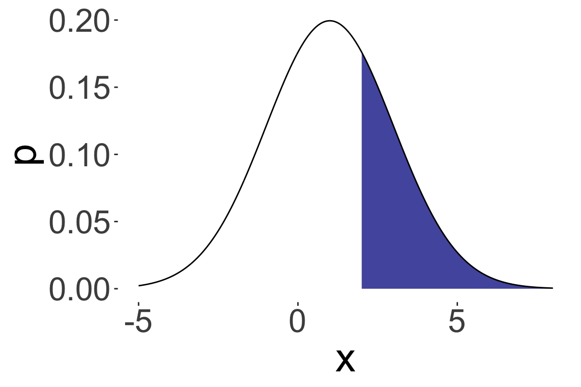
\(P(X > 2)\) where \(X \sim N(1, 2)\)

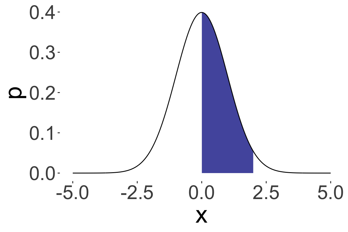
\(P(0 < X < 2)\) where \(X \sim N(0, 1)\)
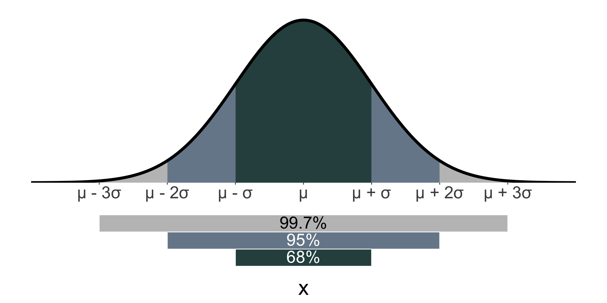
Using standardisation and symmetry

Suppose that you are given the following R output:

pnorm(c(0, 0.5, 1, 1.5, 2, 2.5, 3))
[1] 0.5000000 0.6914625 0.8413447
[4] 0.9331928 0.9772499 0.9937903
[7] 0.9986501

Using the above information only, calculate the following probabilities:

  • \(P(Z < -1)\) where \(Z \sim N(0, 1)\)
  • \(P(X > 1.5)\) where \(X \sim N(1, 1)\)
  • \(P(|X - 1| > 2)\) where \(X \sim N(1, 2)\)
  • If \(X \sim N(\mu, \sigma^2)\), then \[P(X < a) = P\left(Z < \frac{a - \mu}{\sigma}\right)\] where \(Z \sim N(0, 1)\).
  • The normal distribution is symmetric about its mean, i.e. \[P(X < \mu - a) = P(X > \mu + a)\] for any \(a > 0\).

68-95-99.7 rule

  • For a normal distribution, approximately
    • 68% of the population values are within 1 standard deviation of the mean,
    • 95% are within 2 standard deviations of the mean, and
    • 99.7% are within 3 standard deviations of the mean.


E.g. the average adult height is ~167cm, and the standard deviation is ~10cm based on US National Health and Nutrition Examination Survey (2017-2018) data. So assuming the distribution of adult heights is normal, approximately 99.7% of adults have a height between 137cm and 197cm.

Fitting a normal distribution to data

scroll

  • Standing height (in cm) from the US National Health and Nutrition Examination Survey (2017-2018) data.

Student’s t distribution

Student’s t distribution

  • The t-distribution is a continuous distribution that is symmetric and bell-shaped, but has heavier tails than the standard normal distribution.
  • The t-distribution is used when the sample size is small and the population standard deviation is estimated from the sample.
  • The grey area is \(N(0, 1)\) for comparison.
  • As the degrees of freedom increases, the t-distribution approaches the standard normal distribution.
  • \(X \sim t_\nu\) where \(\nu\) is the degrees of freedom.
  • \(E(X) = 0\) for \(\nu > 1\).
  • \(Var(X) = \dfrac{\nu}{\nu - 2}\) for \(\nu > 2\).

t-distribution in R

  • The t-distribution is implemented in R using the dt(), pt(), qt(), and rt() functions, which are analogous to the dnorm(), pnorm(), qnorm(), and rnorm() functions for the normal distribution.

  • When the sample size is large, there is not much difference:

  • However, when the sample size is small, the t-distribution gives a different result:

Summary

Distribution Support Mean Variance
\(X \sim U(a, b)\) \([a, b]\) \(\dfrac{a + b}{2}\) \(\dfrac{(b - a)^2}{12}\)
\(X \sim N(\mu, \sigma^2)\) \((-\infty, \infty)\) \(\mu\) \(\sigma^2\)
\(X \sim t(\nu)\) \((-\infty, \infty)\) \(0\) (for \(\nu > 1\)) \(\frac{\nu}{\nu - 2}\) (for \(\nu > 2\))
Distribution pdf cdf quantile function random generation
Uniform dunif(x, a, b) punif(q, a, b) qunif(p, a, b) runif(n, a, b)
Normal dnorm(x, mean, sd) pnorm(q, mean, sd) qnorm(p, mean, sd) rnorm(n, mean, sd)
t-distribution dt(x, df) pt(q, df) qt(p, df) rt(n, df)
  • The normal distribution is a continuous distribution that is symmetric and bell-shaped, and is used to model many natural phenomena.
  • The t-distribution has heavier tails than the standard normal distribution, and is used when the sample size is small and the population standard deviation is estimated from the sample.