Basic Statistical Concepts and Programming II

STAT1003 – Statistical Techniques

Dr. Emi Tanaka

Australian National University

These slides are best viewed on a modern browser like Google Chrome on a desktop or laptop. Some interactive components may require some time to fully load.

Summary Statistics for Bivariate Data

Bivariate data

Bivariate data involves two different variables (\(x\) and \(y\)) for each observation.

  • Suppose \(x_i\) and \(y_i\) are two variables measured on the same unit \(i\) for \(i = 1, 2, \ldots, n\).
  • It allows us to explore relationships and associations between the two variables.
  • Examples:
    • Height and weight of individuals.
    • Temperature and ice cream sales.
    • Study time and exam scores.
    • Eye color and hair color.
Categorical Numerical
Categorical
  • Contingency table
  • Stacked barplot
  • Percent stacked barplot
  • Side-by-side barplot
  • Group summary statistics
Numerical
  • Group summary statistics
  • Scatterplot
  • Covariance
  • Correlation coefficient

Contingency table

A contingency table (also known as a cross-tabulation or crosstab) display the frequency distribution of two or more categorical variables.

What do you notice between these two approaches?

Stacked barplot

A stacked barplot is used to compare the composition of different groups in a dataset, especially contribution of sub-categories to the total within each main category.

Percent stacked barplot

A percent stacked barplot is ideal for comparing the relative frequencies of subgroups within categories, rather than their absolute counts.

Side-by-side barplot

A side-by-side barplot (also called a grouped barplot) is used to visually compare the values of different subgroups across categories.

Group summary statistics

For a bivariate data where one variable is numerical and the other is categorical, you can use summary statistics for univariate data for each group.

  • For example, numerical statistics for each group can be computed as:

Graphical statistics by group

  • Likewise, we can compute graphical statistics for each group.

Beeswarm plot is a type of scatterplot that shows the distribution of data points while avoiding overlap, making it easier to visualize the density and spread of the data.

Case study 🌾 Wheat seed morphological characteristics

A dataset was collected to investigate morphological characteristics associated with seed weight in a line of diploid wheat (Triticum monococcum).

  • DSeed - identifier for each seed
  • Weight - weight of seed (mg)
  • Length - length of seed (mm)
  • Diameter - diameter of seed (mm)
  • Moisture - mositure content of seed (as a percentage)
  • Hardness - endosperm hardness

Scatterplot

A scatterplot is a graphical representation that displays the relationship between two numerical variables by plotting individual data points on a two-dimensional graph.

Sample covariance

Sample covariance is a measure of how much two numerical variables change together.

\[ s_{xy}=\frac{1}{n-1} \sum_{i=1}^{n}\left(x_{i}-\bar{x}\right)\left(y_{i}-\bar{y}\right) \]

  • Interpretation:
    • When \(s_{xy} > 0\), the variables tend to increase together.
    • When \(s_{xy} < 0\), one variable tends to increase when the other decreases.
    • When \(s_{xy} = 0\), there is no linear relationship between the variables.

Consider the following dataset with two variables, \(x\) and \(y\):

\(i\) \(x\) \(y\)
1 1 10
2 2 70
3 3 100

\[s_{xy} = \frac{1}{2}\left[(1-2)(10-60)+(2-2)(70-60)+(3-2)(100-60)\right]=45\]

  • But the magnitude of covariance is not easy to interpret since it depends on the units of the variables.

Pearson’s correlation coefficient

  • Correlation coefficient is a normalised version of covariance.
  • The sample Pearson correlation coefficient, denoted as \(r\), is a measure of the strength of a linear relationship between two variables (\(x\) and \(y\)).

\[r = \frac{\sum_{i=1}^n(x_i-\bar{x})(y_i - \bar{y})}{\sqrt{\sum_{i=1}^n(x_i - \bar{x})^2\sum_{i=1}^n(y_i - \bar{y})^2}}\]

  • The correlation coefficient ranges from -1 to 1.

Interpretation of correlation coefficient

  • The sign of the correlation coefficient indicates the direction of the relationship.
  • The magnitude indicates the strength of the linear relationship.
\(|r|\) Interpretation
0.8 - 1.0 Very strong association
0.6 - 0.8 Strong association
0.4 - 0.6 Moderate association
0.2 - 0.4 Weak association
0.0 - 0.2 Very weak association

Wrong interpretation of correlation coefficient
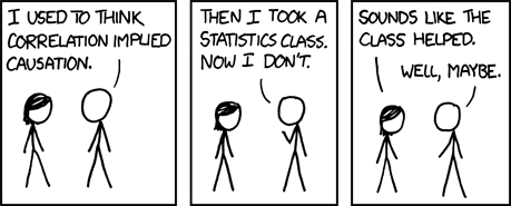

Source: xkcd

Just because \(x\) and \(y\) are highly correlated, it does not mean that \(x\) causes \(y\) or vice versa – correlation is not causation!

  • Number of ice cream sales and the rate of drowning deaths.
  • It is also easy to get spurious correlation if computing many pairwise correlations.
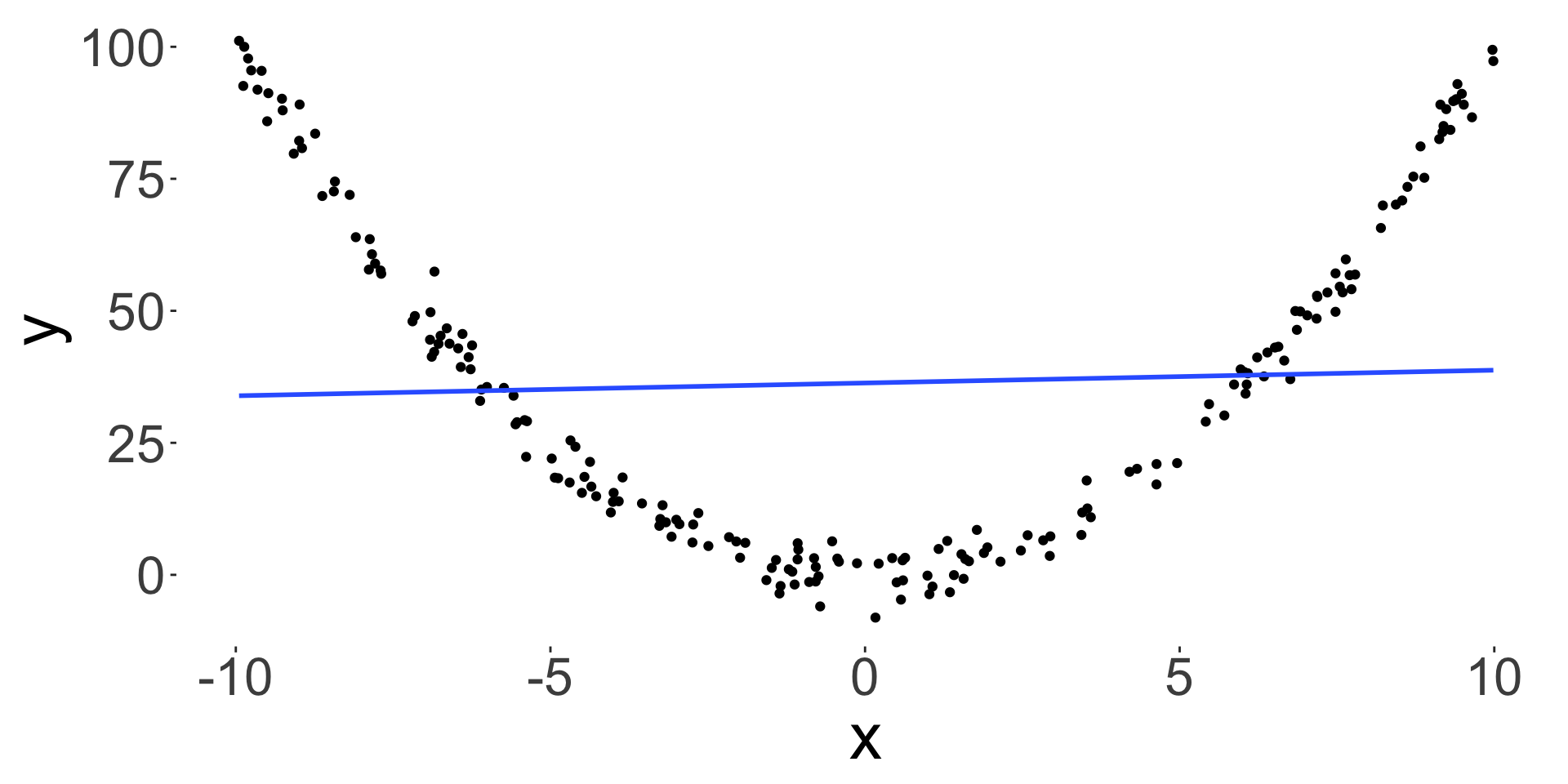
  • Correlation also only measures a linear relationship, so low correlation doesn’t mean that there is no relationship.

\[r = 0.0465043\]

Summary statistics can be misleading

  • You can have a bivariate dataset with the exact same:
    • marginal mean,
    • marginal variance and
    • correlation, but the relationship between the two variables can be very different.
  • Always plot your data!
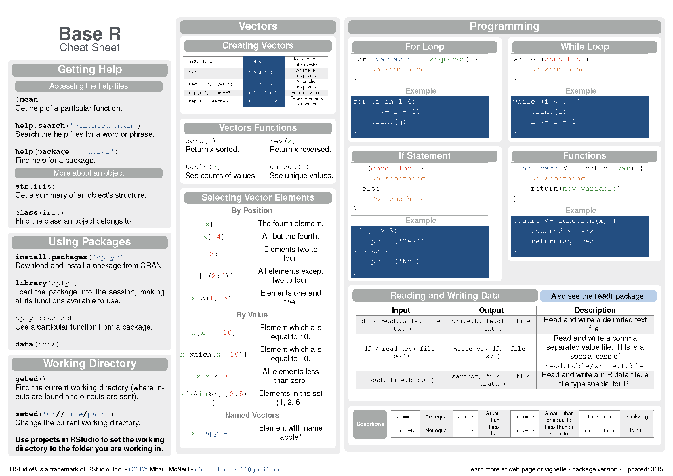
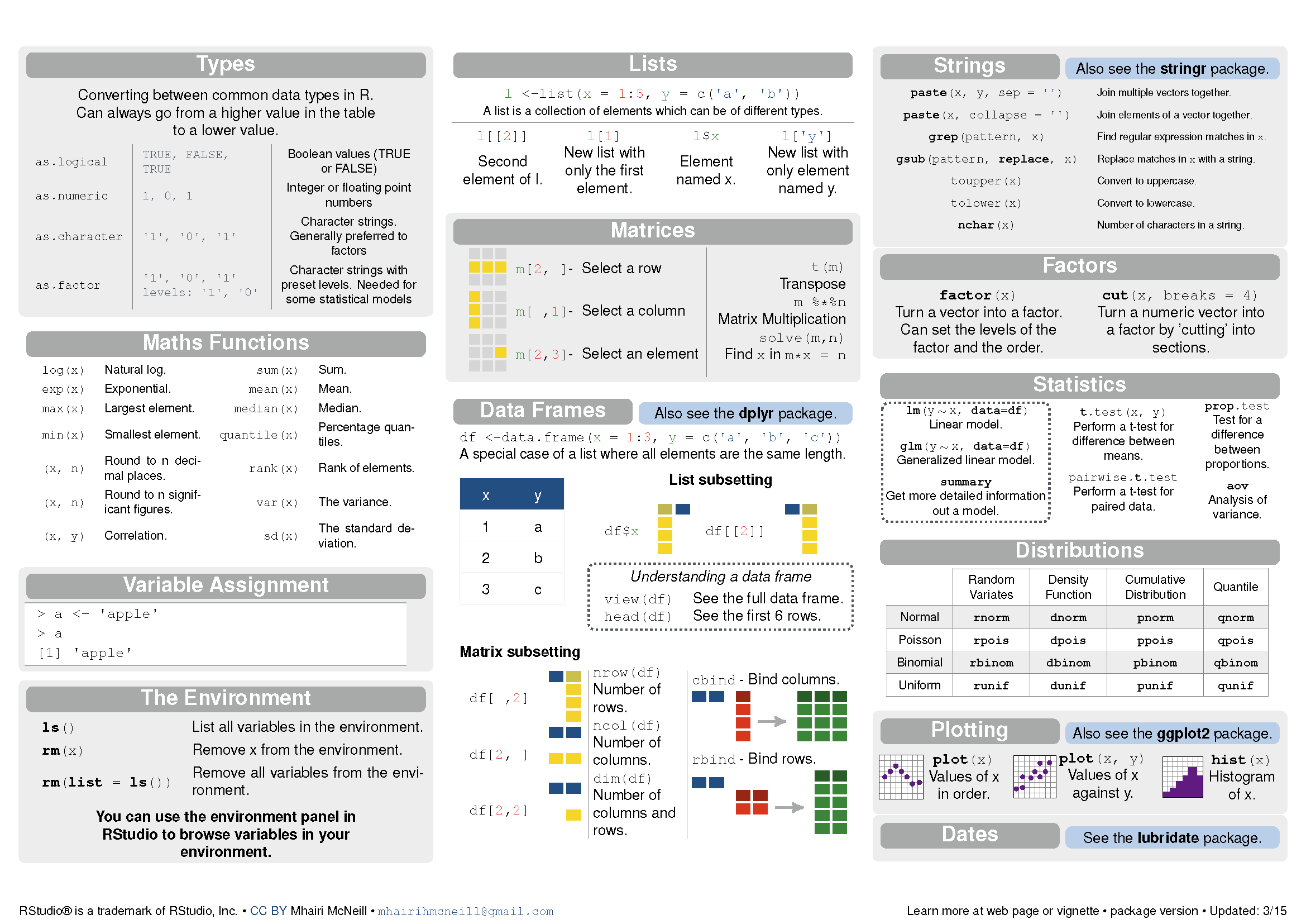
Summary

Categorical Numerical
Categorical
  • Contingency table
  • Stacked barplot
  • Percent stacked barplot
  • Side-by-side barplot
  • Group summary statistics
Numerical
  • Group summary statistics
  • Scatterplot
  • Covariance
  • Correlation coefficient
  • Correlation \(\neq\) Causation
  • Always plot the data!

R Objects

Using R as a calculator

  • \(e^{3 + 4}\)
  • \(e^{3 + 4} + \frac{1}{3}(1 + 3 + 5)\)
  • But we want to save results to reuse later!

Assignment

  • You can assign values to objects using <- or = or even ->
  • Just be consistent which one you use!
  • The name of the object can be variable so long as it is syntactically valid (no spaces and most special characters, and the name cannot start with a digit)

Vectors

  • We can combine scalars to form vectors using c():
  • This is a vector of length 3
  • This vector is stored as a double with the class as numeric

Vector types

There are four primary types of atomic vectors: logical, integer, double and character.

  • If a logical value is coerced to numeric or integer, then
    • TRUE is 1 and
    • FALSE is 0.

Vector coercion

  • A vector can only consist of the same type.
  • If you attempt to combine mismatched types together, it will try to coerce all values to the same type.
  • There are functions to explicitly coerce types, e.g., as.numeric() tries to coerce input to numeric value.

Factor

A factor in R is a special type of integer vector used typically to encode categorical variables.

Lists

  • Lists allow to combine elements of different types.
  • You can use str() to see the internal structure of an object in R.

Data frames

data.frame is a special type of a named list where each element of the vector is the same length.

  • tibble is a Tidyverse version of data.frame in R.
  • It is still a data.frame, so all functions that work with data.frame objects will also work with tibble objects.

Subsetting vectors Part 1

A vector can be subsetted using integers in [].

  • Positive integers select elements at the specified positions:
  • Negative integers exclude elements at the specified positions:

Subsetting vectors Part 2

Logical vectors in [] select elements where logical value is TRUE.

  • If the logical vector used for subsetting a vector is shorter than it then the logical vector is recycled to match the length of the vector.

Subsetting named vectors

Character vectors select elements based on the name of the vector (if any):

Subsetting lists

Lists can be subsetted using integers in [] or names with $ or [[ ]].

Subsetting data frames

A data.frame can be subsetted using integers in [ , ] or names with $ or [[ ]].

Missing values

  • NA in R denotes missing values – there are in fact different types of missing values (NA_character_, NA_integer_, NA_real_, NA_complex_, NA_Date_, NA_POSIXct_).
  • When there are missing values, it can cause issues in the computation.
  • Below we remove the missing values:

Summary

  • Four primary types of atomic vectors: logical, integer, double and character.
  • A vector can only consist of the same type.
  • Other objects types: factor, list, and data.frame.
  • There were several ways of subsetting vectors and lists.
  • Missing values represented as NA and may need to be handled specially.

Base R Cheatsheet

Base R Cheatsheet

Data Wrangling with Tidyverse

Tidyverse

  • Tidyverse refers to a collection of R-packages that share a common (opinionated) design philosophy, grammar and data structure.
  • This trains your mental model to do data science tasks in a manner which may make it easier, faster, and/or fun for you to do these tasks.
  • library(tidyverse) is a shorthand for loading the 9 core tidyverse packages: ggplot2, dplyr, tidyr, readr, tibble, purrr, stringr, forcats, lubridate.

A grammar of data manipulation

  • dplyr is a core package in tidyverse
  • It provides a grammar of data manipulation that is consistent with the tidyverse design philosophy.
  • Similar data manipulation can be achieved with base R but dplyr provides a more consistent and user-friendly interface for data manipulation tasks.
  • The earlier concept of dplyr (first on CRAN in 2014-01-29) was implemented in plyr (first on CRAN in 2008-10-08).
  • The functions in dplyr has been evolving but dplyr v1.0.0 was released on CRAN in 2020-05-29 suggesting that functions in dplyr are maturing and thus the user interface is unlikely to change.

Lifecycle

  • Functions (and sometimes arguments of functions) in tidyverse packages often are labelled with a badge like on the left

Lionel Henry (2020). lifecycle: Manage the Life Cycle of your Package Functions. R package version 0.2.0.

dplyr “verbs”

  • The main functions of dplyr include:
  • arrange
  • select
  • mutate
  • rename
  • filter
  • summarise
  • Notice that these functions are verbs.
  • Functions in dplyr generally have the form:
verb(data, args)
  • The first argument data is a data.frame object.
  • Let’s use the tips data from GGally package to illustrate some of the dplyr functions.
  • What do you think the following will do?

Pipe operator

  • Almost all the tidyverse packages use the pipe operator %>% from the magrittr package.
  • R version 4.1.0 introduced a native pipe operator |> which is similar to %>% but with some differences.
  • x |> f(y) is the same as f(x, y).
  • x |> f(y) |> g(z) is the same as g(f(x, y), z).
  • When you see the pipe operator, read it as “and then”.

Tidyselect

  • Tidyverse packages generally use syntax from the tidyselect package for column selection.

Selection language

  • The selection language in tidyselect can be found in the documentation:

tibble objects

  • tibble is a modern reimagining of the data.frame object.

Subsetting by column via Tidyverse

What’s the difference between these?

Subsetting by row via Tidyverse

What is happening here?

See also filter_out() for filtering out rows by condition for dplyr v1.2.0 or greater.

Adding or modifying a column via Tidyverse

  • You can add new columns or modify existing columns using mutate().
  • For conditional modification, you can use ifelse() or case_when().

Also see recode_values(), replace_values(), and replace_when() for dplyr v1.2.0 or greater.

Sorting columns via Tidyverse

  • You can use select() along with everything() to reorder columns.
  • Similarly, you can use relocate() to move columns around.

Sorting rows via Tidyverse

Calculating statistical summaries by group via Tidyverse

  • The summarise() function allows you to calculate statistical summaries by group.
  • The n() function is a special function that counts the number of observations in each group
    (note: it only works within selective Tidyverse functions).
  • You are recommended to use .by for group operations.

Applying a function to multiple columns via Tidyverse

  • The across() function allows you to apply functions to multiple columns.

Summary

  • Tidyverse packages share a common design philosophy, grammar and data structure.
  • This can train your mental model that is applicable across multiple packages that adopt the Tidyverse design philosophy.
  • The core package dplyr provides a grammar of data manipulation.
  • The main functions in dplyr are verbs that take a data.frame (or tibble) as the first argument.
  • Combining with pipe operator, it can make the code easier to read and write by humans.

dplyr cheatsheet

Debugging

Basic troubleshooting

  • Whether you are good at programming or not, you will inevitably encounter errors.
  • If you encounter an error,

    1. Read the error message!
    2. Google the error message or ask generative AI (like chatGPT)
    3. Ask for help with a reproducible example

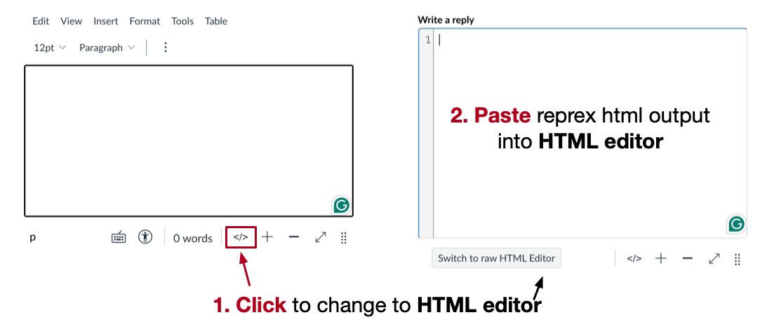
Reproducible Example with reprex LIVE DEMO

  • Copy your minimum reproducible example then run
reprex::reprex(venue = "html")
  • Once you run the above command, your clipboard contains the formatted code and output for you to paste into places like Canvas discussion board