Basic Statistical Concepts and Programming I
STAT1003 – Statistical Techniques
Australian National University
These slides are best viewed on a modern browser like Google Chrome on a desktop or laptop. Some interactive components may require some time to fully load.
What is statistics?
Statistics is defined as the science and technology of obtaining useful information from data, taking its variability into account.
- Statistics involves:
- designing the collection of data,
- organizing data,
- analyzing data,
- developing methods,
- interpreting the results, and
- communicating results.

Why study statistics?
The best thing about being a statistician is that you get to play in everyone’s backyard.
- In a data rich world, statistical literacy is essential for everyone.
- Statistics is essential for making sense of information across fields such as biology, medicine, physics, social sciences, finance, business, and numerous other fields.
- Statistical literacy enables us to think critically and make evidence-based decisions
Newspaper articles from The Australian in January 2026


Become a data detective
Technical proficiency (understand statistical methods and skilled with statistical software for extracting and analyzing data) alone isn’t enough for practice. Think holistically.
- Curiosity: Naturally inquisitive and eager to explore the “why” behind data anomalies or trends.
- Problem-solving skills: Resourceful and persistent in finding solutions and overcoming data challenges.
- Attention to detail: Notices subtle patterns, inconsistencies, or outliers others might miss.
- Critical thinking: Evaluates information objectively, questioning assumptions and sources, and have a healthy dose of skepticism.
- Communication abilities: Clearly conveys insights and explanations to technical and non-technical audiences.
- Ethical judgment: Handles data responsibly and respects privacy and security considerations.
- Collaboration: Works well with colleagues from different domains.
- Project management: Organizes work efficiently, sets goals, and meets deadlines during investigations.

Population vs. Sample
Populations have parameters: a descriptive measure of a population that is usually unobservable and unknown.

Sample statistics are estimated from sample data and used to make inferences about population parameters.
- Ideally, we would measure every single unit of interest (e.g. marks of every STAT1003 student).
- But this is often impractical or unavailable (we only have the 2025 data).
- Instead, a (representative) sample from the population is used to make inference of the population.
Mathematical setup
How hard is STAT1003 at ANU for a typical undergraduate student as measured by the average final grade earned by students in STAT1003?

Population vs sample mean

Let \(\mu\) denote the population mean (average) final grade of all STAT1003 students. \[\begin{align*} \mu &= \frac{1}{N}(x_{1'} + x_{2'} + \dots + x_{N'}) = \frac{1}{N}\sum_{i=1}^{N} x_{i'}\\ &= {\tiny \frac{1}{14}(73 + 60 + 54 + 62 + 71 + 68 + 57 + 60 + 72 + 57 + 35 + 53 + 58 + 70)} \approx 60.7\\ \end{align*}\]
Let \(\bar{x}\) denote the sample mean (average) final grade of the sampled STAT1003 students. \[\begin{align*} \bar{x} &= \frac{1}{n}(x_1 + x_2 + \dots + x_n) = \frac{1}{n}\sum_{i=1}^{n} x_i\\ &= {\tiny \frac{1}{5}(54 + 71 + 57 + 70 + 53)} = 61\\ \end{align*}\]
\(\bar{x}\) is used to estimate \(\mu\).
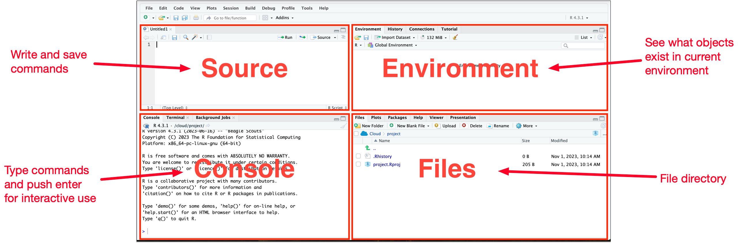
What is R?
- R is a programming language predominately for data analysis.
- RStudio Desktop is an integrated development environment (IDE) that helps you to use R.
![]()
- Visual Studio Code and Positron are other popular IDEs.
How do you use R?
- RStudio Desktop (or RStudio IDE) is the most common way to use R.
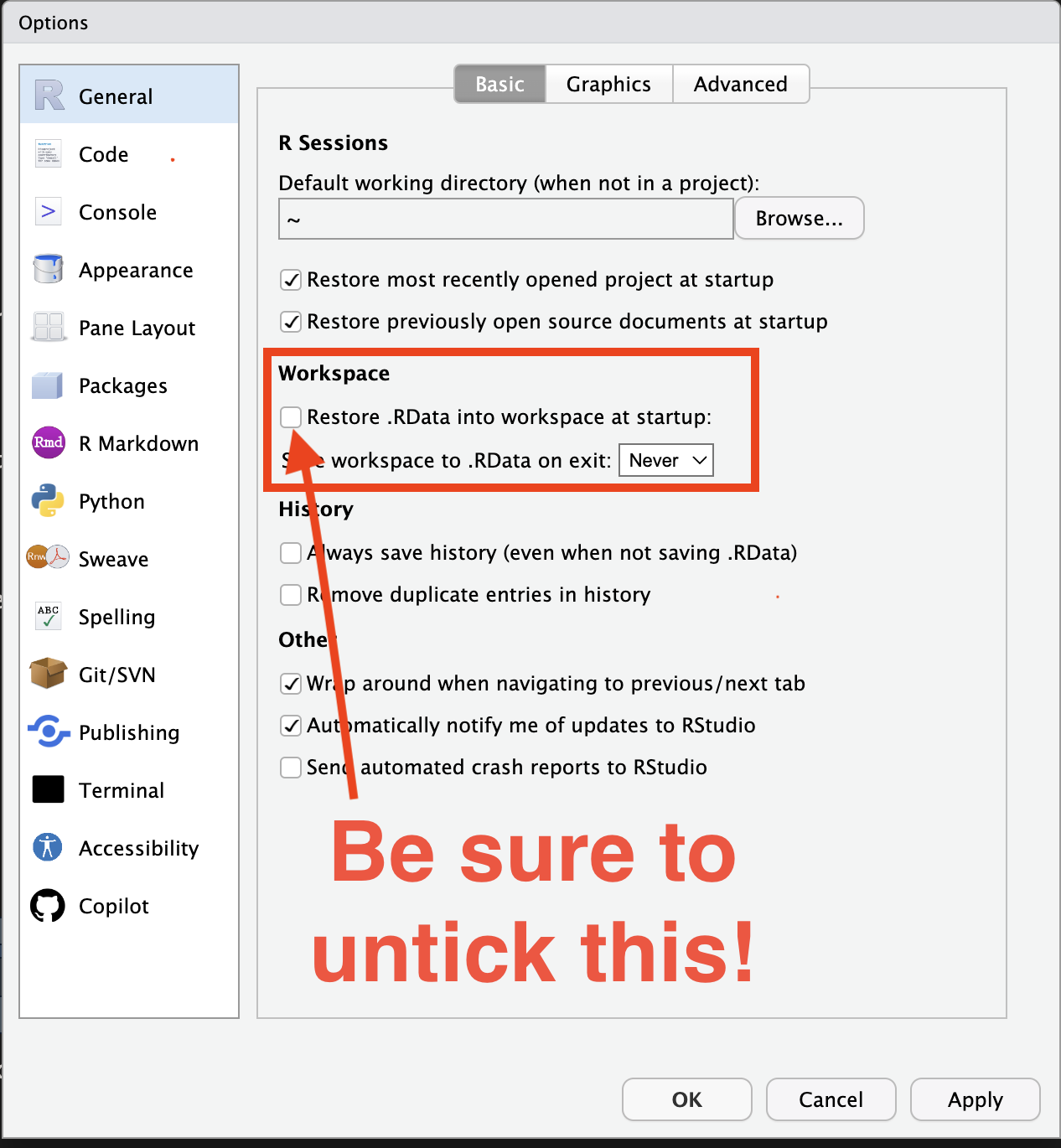
Customise Global Options
- Go to RStudio > Tools > Global Options…
- Under the General tab, make sure the “Restore .RData into workspace at startup” is unticked.
- This avoids unexpectedly loading (old) data into your workspace and making your code only work in your workspace, but not for others (which is bad reproducible practice).
Base R
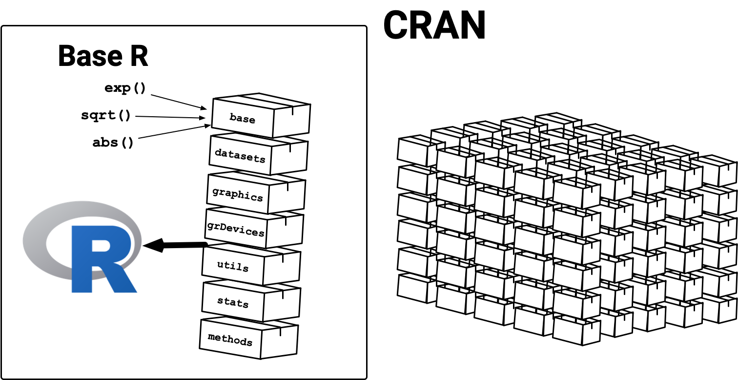
R has 7 packages:
base,datasets,graphics,grDevices,
utils,stats,methods,
collectively referred to as “Base R”, that are loaded automatically when you launch it.
- The functions in the base packages are generally well-tested and trustworthy.
Contributed R Packages
- R packages are community developed extensions to R (much like apps on your mobile).
- The Comprehensive R Archive Network (CRAN) is a volunteer maintained repository that hosts submitted R packages that are approved (much like an app store).
- There are close to 20,000 packages available on CRAN but the qualities of R packages vary.
- There are other repositories that host R packages, e.g. Bioconductor for bioinformatics, R Universe, R-Forge, GitHub (we won’t cover these).

Photo by Sara Kurfeß on Unsplash
Summary
RStudio Desktop (or RStudio IDE)
Console or Source
- Use
?functionorhelp(function)to look at the function documentation - Use
install.packages()to install a package (only once). - Use
library()to load a package. - Use
package::function()to use a function from a package without loading it.
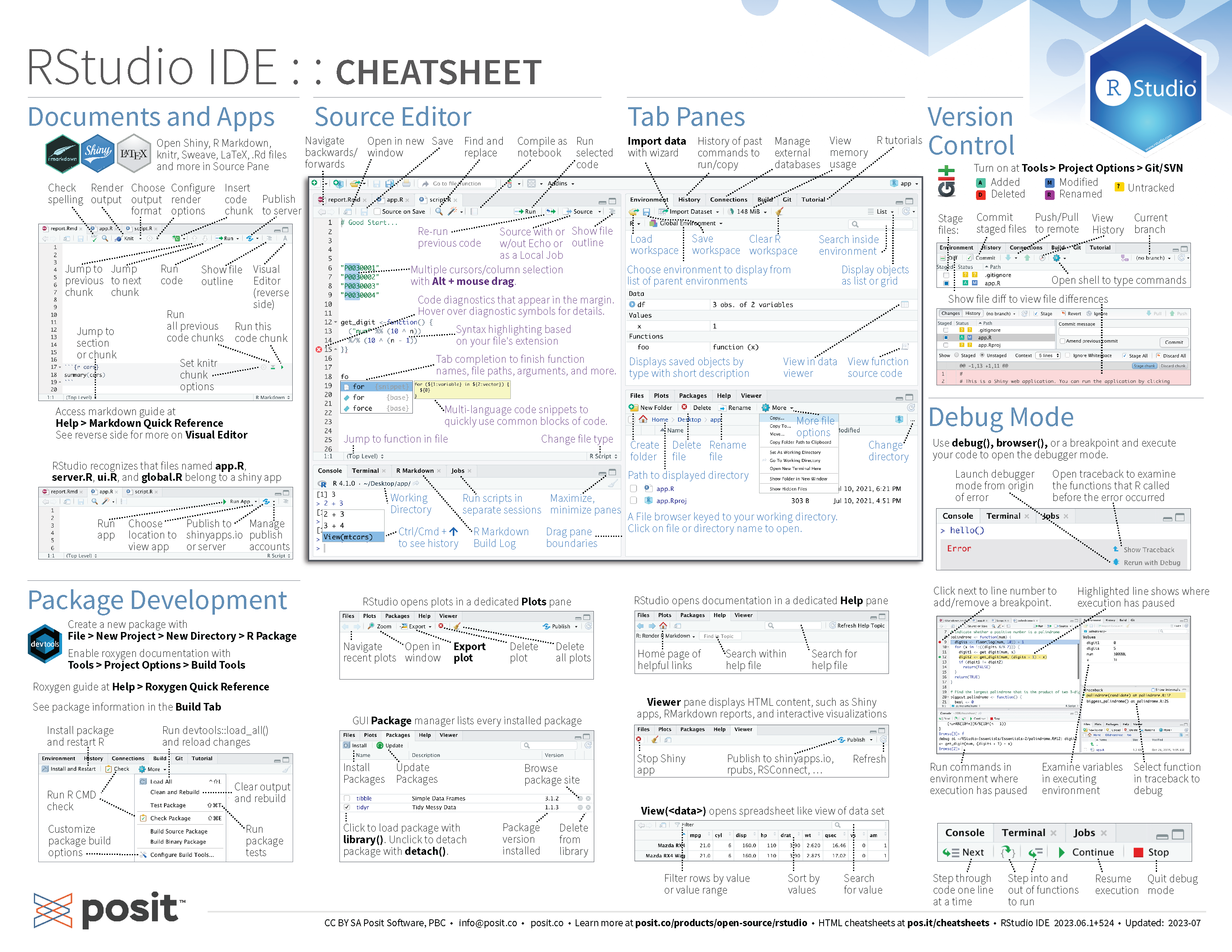
RStudio Desktop Cheatsheet
Nominal vs. Ordinal variables
- We can use exactly the same statistics for ordinal data we used for nominal data, e.g., frequency tables, bar charts, pie charts, etc.
- For ordinal data, preserve the order of the categories.
- For nominal data, reorder the categories based on another variable (if appropriate).
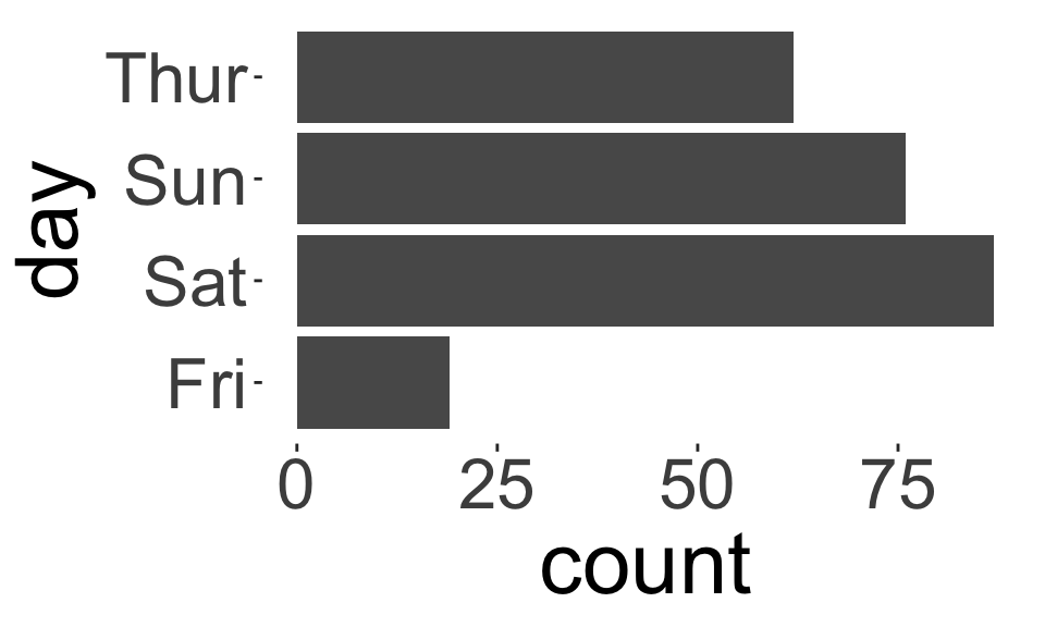
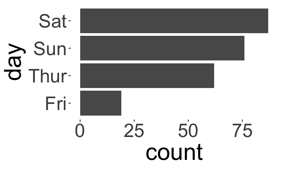
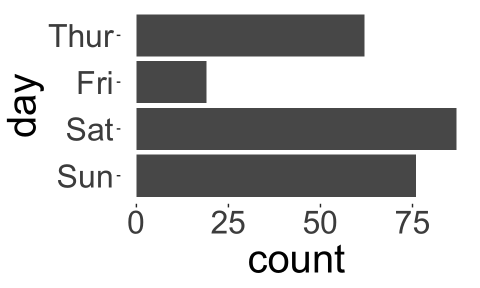
How do these plots differ?
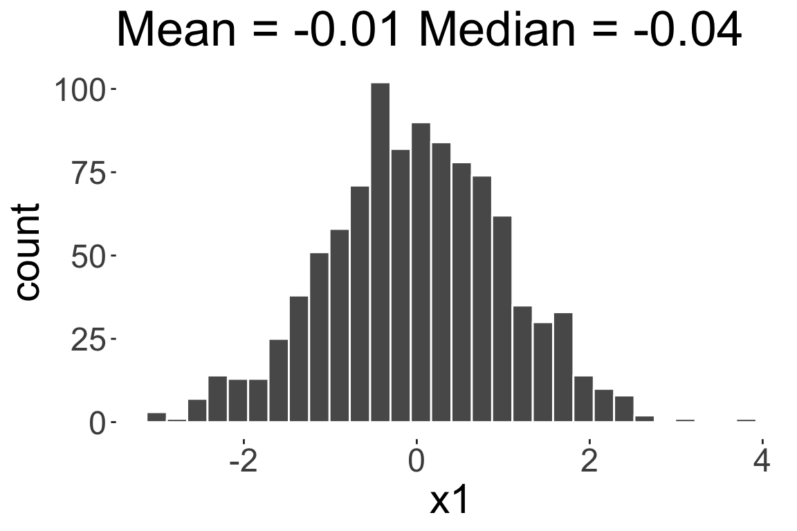
A measure of central tendency
A measure of central tendency is a location of the “middle”, “center”, or “expected value” of the distribution of your data.

Sample mean (or average) and median are examples of measures of central tendency
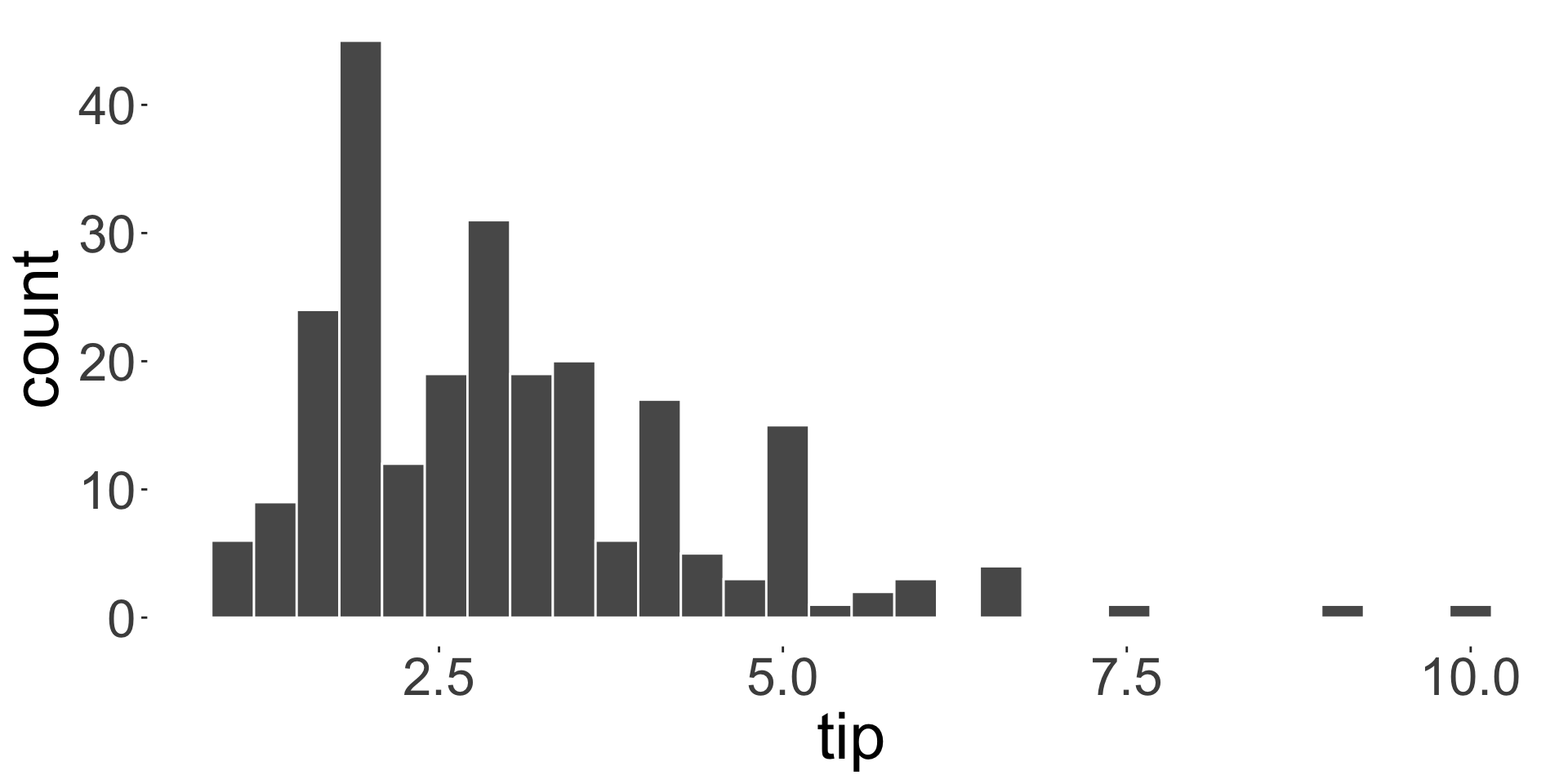
What is the average customer tip?
Skewness
- Skewness is a measure of asymmetry in a given distribution
Symmetric
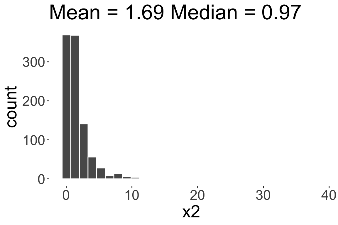
Positively skewed or
Right skewed
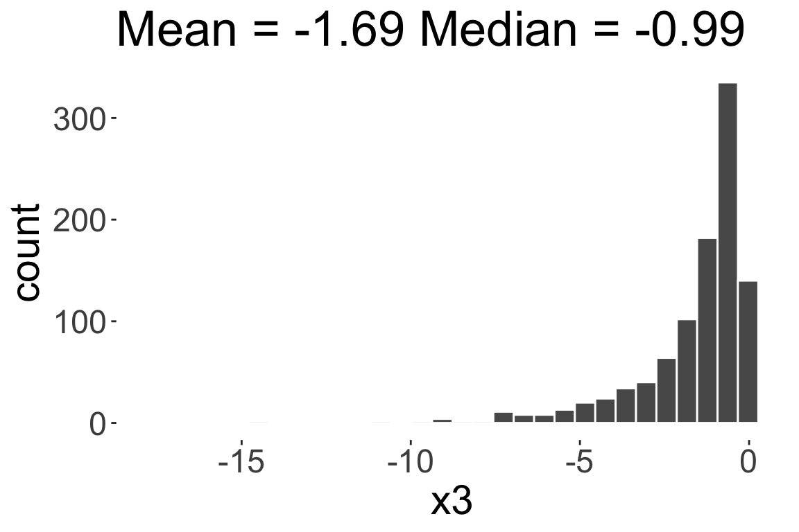
Negatively skewed or
Left skewed
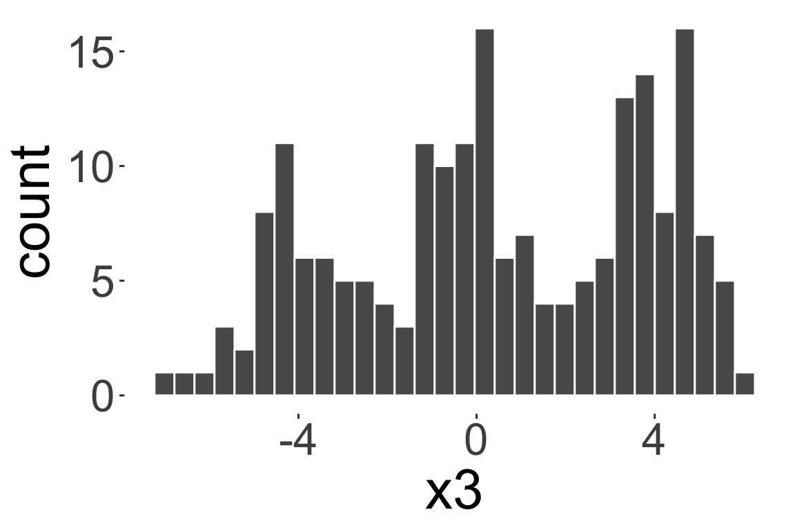
Modality
The sample mode is the value with the highest frequency.
- Mode is useful for categorical data.
- For numerical data, mode is less useful as there may be no repeated values.
- However, we can look at the modality of a distribution: number of peaks in the distribution.
Unimodal distribution
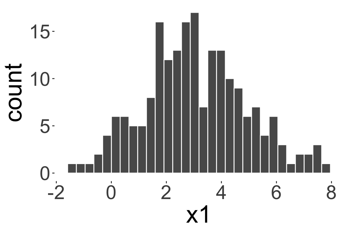
Bimodal distribution
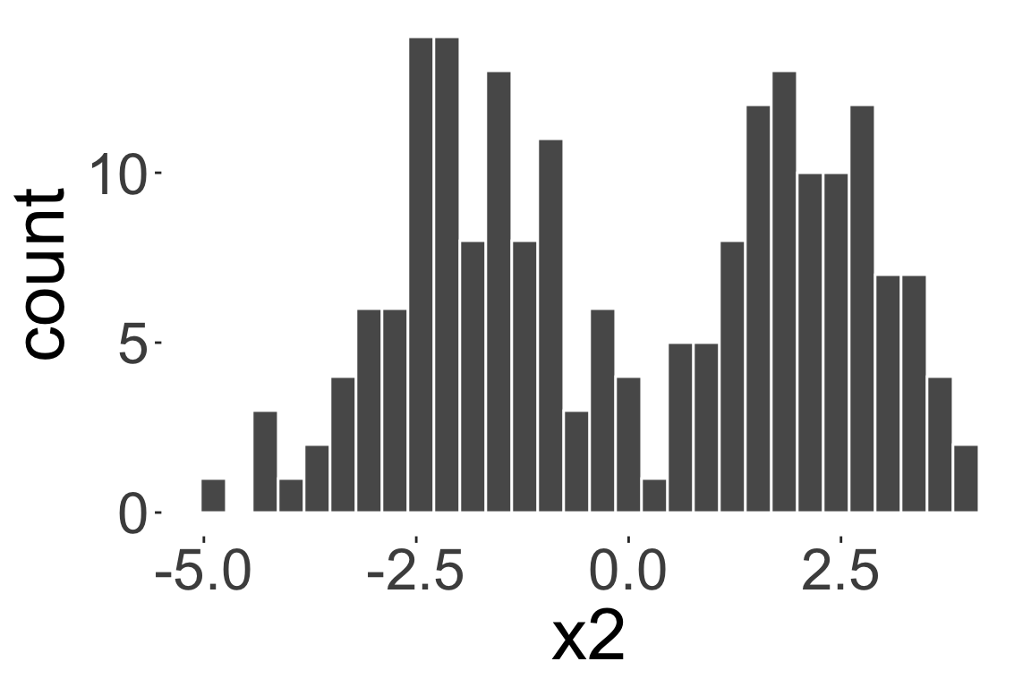
Multimodal distribution
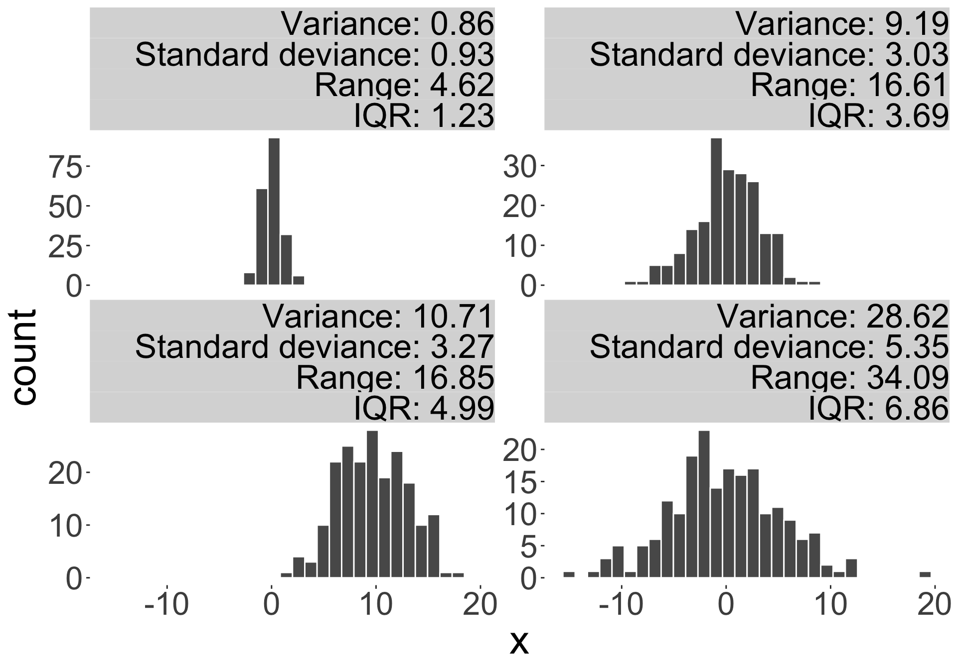
A measure of dispersion
A measure of dispersion/spread is a number representing the spread of data around a measure of central tendency.
- E.g. range, interquartile range (IQR), variance, standard deviation.
Measure of dispersions
- Sample deviation: the distance of an observation from its mean \(x_i-\bar{x}\)
- Sample variance: \[s^2 = \frac{1}{n-1}\sum_{i=1}^n (x_i - \bar{x})^2.\]
- Sample standard deviation: the square root of sample variance \(s\)
- Conveys similar information as variance, but measure of units is the same as the data
- The range is the difference between the maximum and minimum values in the dataset.
- The interquartile range (IQR) is the difference between the third quartile and the first quartile (\(Q_3 - Q_1\)).
Population variance: \[\sigma^2 = \frac{1}{N}\sum_{i=1}^{N} (x_{i'} - \mu)^2.\]
Boxplots

L = \(Q_1 - 1.5 \times IQR\)
U = \(Q_3 + 1.5 \times IQR\)
- Boxplot do not work well for small datasets and certainly not for \(n < 5\).
- Boxplots are poor at showing multimodal distributions.
Case study STAT1003 mark distribution
How hard is STAT1003 at ANU for a typical undergraduate student?
Here is a sample assignment and quiz marks:
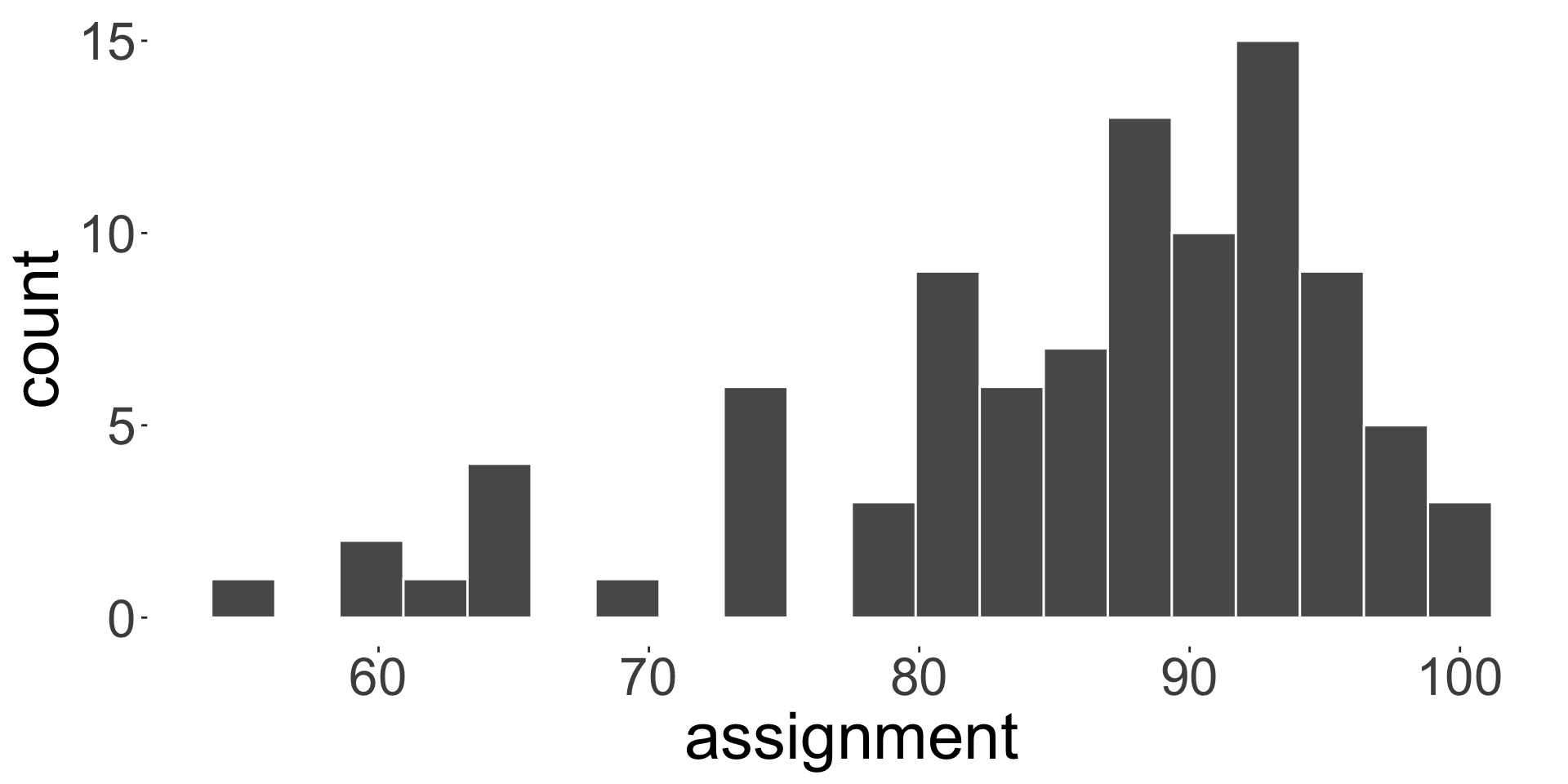
Five number summary: (55, 80, 88, 93, 100)
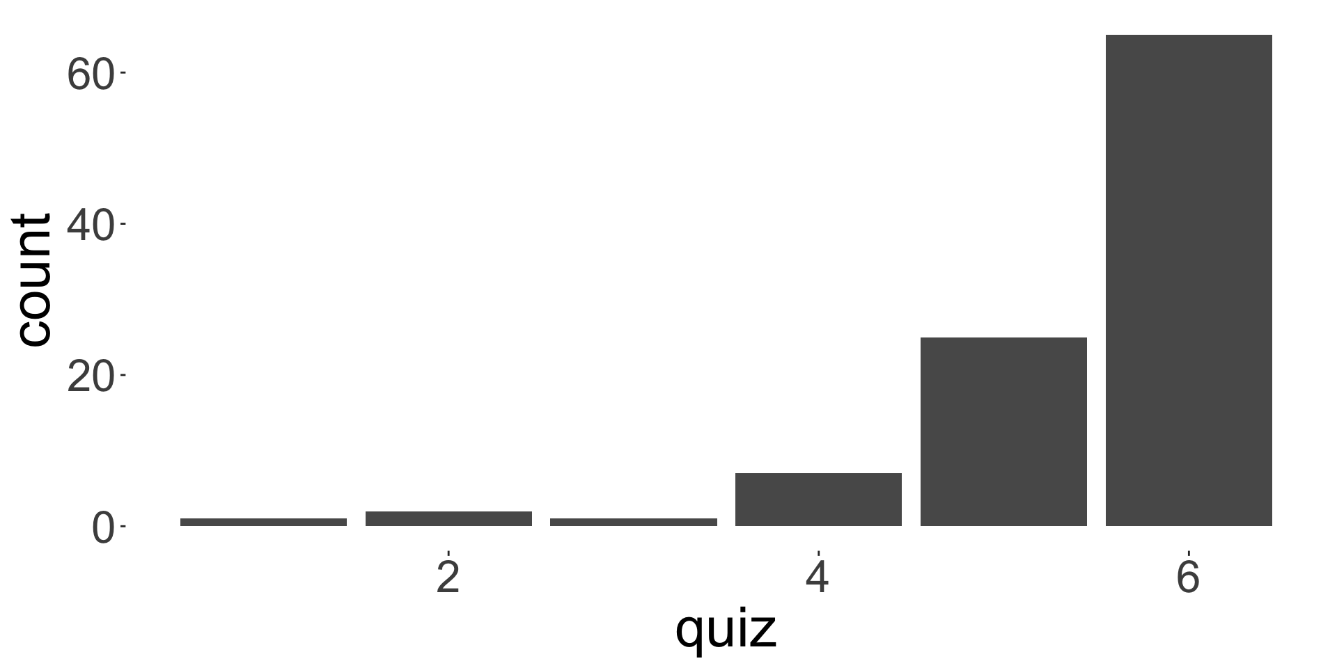
Mode: 6
- Note: five number summary is (minimum, \(Q_1\), median, \(Q_3\), maximum)
- What do you think based on the distribution of marks for assignment and quiz?